Solving The Schrödinger Equation#
We assume you have worked through Ordinary Differential Equations (ODEs) and are familiar with the approach taken there to solve the Schrödinger equation. Here we focus on developing a good set of software for solving this problem more generally.
Here we present a comprehensive worked example of developing a framework for solving the Schrödinger equation. This follows a lot of structures and methodologies developed in our GPE project which solves the Gross-Pitaevskii Equation (GPE) or non-linear Schrödinger Equation (NLSEQ) for superfluid dynamics.
Test Problem#
Following recommendation PP41: Test to Code, we first would like to identify a test problem. We choose the 1D quantum harmonic oscillator since we know it has exact solutions:
This problem is characterized by the following scales, which we take to be unity, defining our units:
\(T = \frac{2\pi}{\omega}\): The trap period, which defines our units of time.
\(a_0 = \sqrt{\hbar/m\omega}\): The trap length, which defines our units of distance.
\(m\): The mass of the particle, which defines our units of mass.
Some facts that are easily checked by substitution into the Schrödinger equation are that the ground state is
Another useful fact is that all motion is periodic with period \(T\). Thus, for any state \(\psi(x, t)\), we have \(\psi(x, t+nT) = \psi(x, t)\). This provides us with an easy test-case. We will evolve some initial state – say the shifted ground state – for one period, and see how close we get to where we started.
As a byproduct, by trying to write this test, we might gain some insight into how we would like to design our Schrödinger equation solver.
Do It! Write a test function.
Write a function to test your desired code using the above invariant. How would you like to interact with your code? What functions do you need?
from scipy.integrate import solve_ivp


def test_ho(seq, x0=2.0):
    a0 = np.sqrt(seq.hbar / seq.m / seq.w)
    T = 2*np.pi / seq.w
    x = seq.x
    psi0 = np.exp(-((x-x0)/a0)**2/2)
    psi1 = seq.evolve(psi0, t=T)
    assert np.allclose(abs(psi0)**2, abs(psi1)**2, rtol=1e-4, atol=1e-4)


class SEQ:
    """Class to help solve the Schrodinger equation for a harmonic trap.

    Attributes
    ----------
    hbar, m, T, w : float
        Various physical constants for the system.
    N : int
        Number of points to include in the lattice
    L : float
        Box size

    """
    hbar = 1.0
    T = 1.0
    m = 1.0
    w = 2*np.pi / T

    def __init__(self, N=64, L=10.0):
        self.N = N
        self.L = 10.0
        self.dx = self.L/self.N
        self.x = np.arange(self.N) * self.dx - self.L/2.0

    def evolve(self, psi, t, **kw):
        """Return `psi(t)` evolving `psi` for time `t`."""
        return psi  # Wrong - but quickly get our tests to pass.


test_ho(SEQ())
Now let’s do a non-trivial implementation based on Ordinary Differential Equations (ODEs):
class SEQ1(SEQ):
    def __init__(self, **kw):
        super().__init__(**kw)
        self.init()

    def init(self):
        D2 = self.get_D2()
        K = -self.hbar**2 / 2 / self.m * D2
        Vx = (self.w * self.x)**2 / 2 / self.m
        V = np.diag(Vx)
        self.H = K + V

    def get_D2(self):
        """Return a matrix approximation for the laplacian."""
        ones = np.ones(self.N)
        D2 = (
            np.diag(ones[1:], 1)
            + np.diag(ones[1:], -1)
            - 2*np.diag(ones)
            ) / self.dx**2
        return D2

    def compute_dy_dt(self, t, psi):
        """Return dpsi_dt."""
        Hpsi = self.H @ psi
        dpsi_dt = Hpsi / (1j * self.hbar)
        return dpsi_dt

    def evolve(self, psi, t, method="DOP853", **kw):
        """Return `psi(t)` evolving `psi` for time `t`."""
        res = solve_ivp(self.compute_dy_dt, y0=psi+0j, t_span=(0, t),
                        method=method, **kw)
        assert res.success
        psi1 = res.y[:, -1]
        self._psi0, self._psi1 = psi, psi1
        return psi1


test_ho(SEQ1(N=128))
---------------------------------------------------------------------------
AssertionError                            Traceback (most recent call last)
Cell In[3], line 39
     35         self._psi0, self._psi1 = psi, psi1
     36         return psi1
---> 39 test_ho(SEQ1(N=128))

Cell In[2], line 10, in test_ho(seq, x0)
      8 psi0 = np.exp(-((x-x0)/a0)**2/2)
      9 psi1 = seq.evolve(psi0, t=T)
---> 10 assert np.allclose(abs(psi0)**2, abs(psi1)**2, rtol=1e-4, atol=1e-4)

AssertionError:
To better understand why the test is not passing, let’s compute the errors:
def get_err(N=256, L=10.0, x0=2.0, SEQ=SEQ1, **kw):
    s = SEQ(N=N, L=L)
    a = np.sqrt(s.hbar / s.m / s.w)
    psi0 = np.exp(-((s.x-x0)/a)**2/2)
    psi1 = s.evolve(psi0, t=s.T, **kw)
    return (abs(psi0)**2 - abs(psi1)**2).max()


Ns = 2**np.arange(2, 9)
errs = [get_err(N=N, SEQ=SEQ1) for N in Ns]
Perhaps a higher order stencil will help. Here we try the 5-point stencil from Derivatives:
class SEQ2(SEQ1):
    def get_D2(self):
        """Return a matrix approximation for the laplacian."""
        # 5-point stencil
        stencil = np.array([-1, 16, -30, 16, -1])/12
        k = [-2, -1, 0, 1, 2]
        ones = np.ones(self.N)
        D2 = np.sum([s * np.diag(ones[abs(k):], k)
                     for (s, k) in zip(stencil, k)], axis=0)
        return D2 / self.dx**2


test_ho(SEQ2(N=256, L=10.0), x0=1.0)
This works, but we should probably think a little about why. The IR errors are due to the box, and should be largest at the boundary, so we can estimate the error to be roughly:
For \(L=10\) and \(x_0=2.0\), this is below \(3\times 10^{-25}\) so we should be fine, and we can probably reduce the box size to \(L=8\) without any worry.
To estimate the UV errors, we note that the truncation error in our approximation of the derivative is
To estimate \(f^{(4)}\) we note that a particle moving with definite momentum \(p\) will have wavefunction \(\psi(x) \propto e^{\I p x/\hbar}\), so \(\psi^{(n)}(x) \sim (p/\hbar)^n\). The relative error is the ratio of the two terms, thus
We can estimate the momentum from conservation of energy. With \(x_0=2.0\) and \(L=10.0\), we have
Thus, to get \(\epsilon \sim 10^{-4}\), we would need \(N \gtrsim 3600\) points. Repeating this analysis for the 5-point stencil gives
hence, reducing \(x_0 = 1.0\) and using \(N=256\) points gives \(\epsilon \sim 4\times 10^{-5}\): our test passes.
Spectral Methods#
We can get a much better approximation for the derivative by using the Fourier transform (see Fourier Techniques). The idea here is to write \(\psi(x)\) as a sum of plane-waves \(e^{\I k x}\) so that, to compute the second derivative, we simply multiply by \(-k_n^2\) in momentum space.
The only thing remaining is to get the appropriate \(k_m\) in the correct order, which we
do by calling numpy.fft.fftfreq().
N = 64
L = 18.0
dx = L/N
n = np.arange(N)
x = n * dx - L/2
k = 2*np.pi * np.fft.fftfreq(N, dx)

def diff(f, d=2):
    """Return the dth derivative of f."""
    return np.fft.ifft((1j*k)**d * np.fft.fft(f))
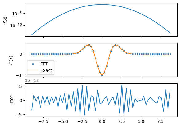
We see in the margin that we can reach machine precision with \(N=64\) points with a large enough box \(L=18\). This is about optimal for this problem as we can see by computing the analytic Fourier transform of our gaussian:
To achieve precision \(\epsilon = 2^{-52} \approx 2\times 10^{-16}\), these functions must drop by this amount at the edge of the box \(x=\pm L/2\) and for the largest wave-numbers \(k = \pm \pi N/L\):
Note
These estimates are a little low for \(f''(x)\) where we should use
Evaluating these at the edge of the box gives \(L, 2k \gtrapprox 18\) and \(N \gtrapprox 52\). Playing a bit with the code, to achieve maximum precision we really need \(N \gtrapprox 64\) – do you see why?