Model Fitting E.g. 1b: MCMC#
We continue our example of fitting a cosine, but now in the case where we have large errors, so that the model is certainly not linear.
In this case, the posterior will not be gaussian, and to properly characterize it, we will need to use Markov chain Monte Carlo (MCMC). We will use the emcee package, but many others exists. See the following for a summary:
Samples, samples, everywhere…: A nice overview of different MCMC software accessible with python.
Recall that, from the Bayesian perspective, our goal is to compute the posterior probability distribution
where \(p(\vect{a})\) is the prior, \(\mathcal{L}(\vect{a}|\vect{y}) = p(\vect{y}|\vect{a})\) is the likelihood, and \(p(\vect{a}|\vect{y})\) is our desired posterior. We will still use independent errors:
but will not assume these to always be gaussian.
All that emcee needs is a function log_prob(p) which returns the log of the posterior:
The last normalization constant need not be included. The MCMC method will then generate a sample which approximates the correct distribution.
For our curve-fitting model:
For gaussian errors, \(\rho(x) = -\ln N(x) = x^2/\sqrt{2\pi}\).
from IPython.display import Latex
from collections import namedtuple
from uncertainties import correlated_values, unumpy as unp
from scipy.optimize import least_squares
from scipy.stats import chi2
import emcee

Nt = 12
#Nt = 100
t_max = 10.0

# Exact parameter values
Params = namedtuple("Params", ["w", "c", "A", "phi"])
a_exact = Params(w=2 * np.pi / 5, c=2.1, A=3.4, phi=5.6)
w, c, A, phi = a_exact
labels = Params(*map("${}$".format, [r"\omega", "c", "A", r"\phi"]))


def f(t, w, c, A, phi, np=np):
    """Model function."""
    return c + A * np.cos(w * t + phi)


# Exact data and experimental errors
t = np.linspace(0, t_max, Nt)
y = f(t, *a_exact)
sigmas = 0.5 * np.ones(Nt)


# Randomly generated data... An "Experiment"
rng = np.random.default_rng(seed=2)
ydata = rng.normal(loc=y, scale=sigmas)

def rho(e):
    return e**2/np.sqrt(2*np.pi)

def log_liklihood(a, xdata, ydata, sigmas):
    es = (ydata - f(xdata, *a))/sigmas
    return - rho(es).sum() - np.log(sigmas).sum()

def log_prior(a):
    """Uniform prior."""
    return 1

def log_prob(a, *v, **kw):
    return log_prior(a) + log_liklihood(a, *v, **kw)

def get_residuals(p, xdata=t, ydata=ydata, sigmas=sigmas):
    """Return residuals for least_squares."""
    return (ydata - f(xdata, *p))/sigmas

args = (t, ydata, sigmas)

ts = np.linspace(0, t_max)  # Many points for a smooth curve.
fig, ax = plt.subplots(figsize=(10, 5))
ax.errorbar(t, ydata, yerr=sigmas, fmt="C0.", ecolor="C1", label="data")
ax.plot(ts, f(ts, *a_exact), "-C2", label="exact")
ax.set(xlabel="$t$", ylabel="$f(t)$")
ax.legend();
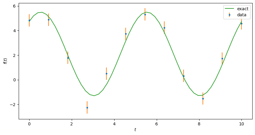
Now we do the fits. We start with the standard least-square fit, then use that as a seed for the emcee code.
res = least_squares(fun=get_residuals, x0=a_exact, jac='cs', args=args)
p = Params(*res.x)
C = np.linalg.inv(res.jac.T @ res.jac)
r = get_residuals(p)
nu = len(r) - len(p)
chi2_r = np.sum(abs(r)**2) / nu
Q = 1 - chi2.cdf(chi2_r*nu, df=nu)

Latex(rf"$\chi^2_r = {chi2_r:.2g}, \qquad Q = {Q:.2g}$")

nwalkers = 32
sampler = emcee.EnsembleSampler(nwalkers=nwalkers, ndim=len(p), log_prob_fn=log_prob, args=args)

# Generate initial set of walkers using a gaussian with the least_sqares
# estimates for the mean (best fit values) and covariance matrix
p0 = rng.multivariate_normal(mean=p, cov=C, size=nwalkers)


state = sampler.run_mcmc(p0, 100)  # Burn-in period of 100 steps
sampler.reset()
%time state = sampler.run_mcmc(p0, 10000)  # Actual run with 10000 walkers
CPU times: user 6.57 s, sys: 9.27 ms, total: 6.58 s
Wall time: 6.58 s
import corner
%load_ext autoreload
%autoreload
import phys_581.plotting
from phys_581.plotting import corner_plot

flat_samples = sampler.get_chain(discard=100, thin=15, flat=True)
fig = corner.corner(flat_samples, labels=labels)
axes = np.array(fig.axes).reshape((4,4))
corner_plot(p, C, axes=axes);
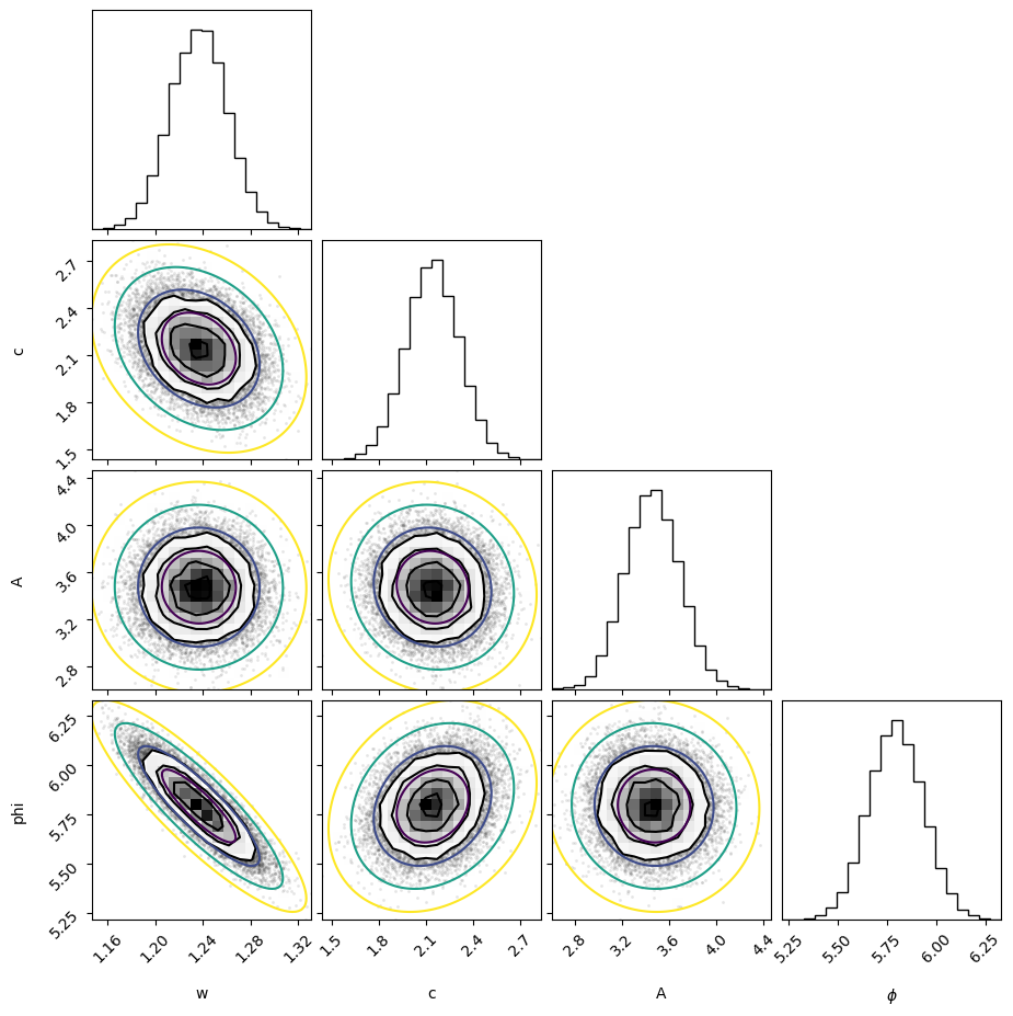
Now we repeat the exercize, but with much larger errors - well beyond the regime where the model is linear.
sigmas = 1.5 * np.ones(Nt)

# Randomly generated data... An "Experiment"
rng = np.random.default_rng(seed=2)
ydata = rng.normal(loc=y, scale=sigmas)

args = (t, ydata, sigmas)


res = least_squares(fun=get_residuals, x0=a_exact, jac='cs', args=args)
p = Params(*res.x)
C = np.linalg.inv(res.jac.T @ res.jac)
r = get_residuals(p)
nu = len(r) - len(p)
chi2_r = np.sum(abs(r)**2) / nu
Q = 1 - chi2.cdf(chi2_r*nu, df=nu)

Latex(rf"$\chi^2_r = {chi2_r:.2g}, \qquad Q = {Q:.2g}$")

nwalkers = 100
sampler = emcee.EnsembleSampler(nwalkers=nwalkers, ndim=len(p), log_prob_fn=log_prob, args=args)

p0 = rng.multivariate_normal(mean=p, cov=C, size=nwalkers)

%time state = sampler.run_mcmc(p0, 10100)  # Actual run with 10000 walkers

flat_samples = sampler.get_chain(discard=2500, thin=15, flat=True)
fig = corner.corner(flat_samples, labels=labels)
axes = np.array(fig.axes).reshape((4,4))
corner_plot(p, C, axes=axes);
CPU times: user 15.1 s, sys: 17.1 ms, total: 15.1 s
Wall time: 15.1 s
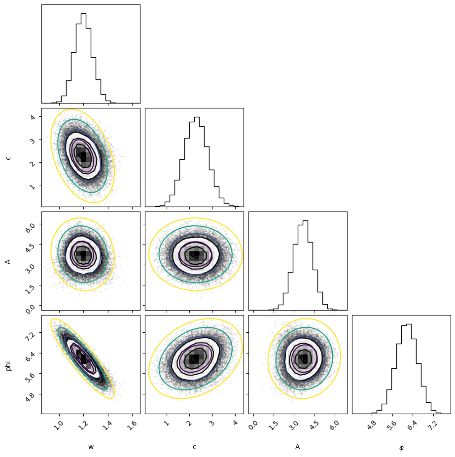
We see some interesting features here. In particular, additional regions are appearing which we did not consider before. Inspecting a bit more closely, we see that one such region is related to our main region by \(A \rightarrow -A\) and \(\phi \rightarrow \phi \pm \pi\). This is completely expected since our model has many discrete degeneracies. We could cure this by introducing a prior that limits the range of the parameter.
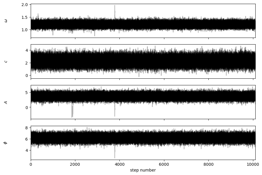
Many other issues, such as determining how many walkers to use, how long a burn-in period is required, etc., should also be studied. See the emcee documentation for details.
fig, axs = plt.subplots(4, figsize=(10, 7), sharex=True)
samples = sampler.get_chain()
for i in range(len(p)):
    ax = axs[i]
    ax.plot(samples[:, :, i], "k", alpha=0.3)
    ax.set_xlim(0, len(samples))
    ax.set_ylabel(labels[i])
    ax.yaxis.set_label_coords(-0.1, 0.5)

axs[-1].set_xlabel("step number");