Derivatives#
Finite Differences#
A straightforward way of computing derivatives is to use finite difference formula, derive from the Taylor series:
The simplest of these are:
5-point stencil for \(f''(x)\).
To improve precision, a 5-point stencil [-1, 16, -30, 16, -1]/12 for computing
\(f''(x)\) is useful. To simplify notation, we write \(f_{n} = f(x+nh)\):
import sympy
x, h = sympy.var('x, h')
f = sympy.Function('f')
f2 = (-(f(x+2*h) + f(x-2*h)) + 16 * (f(x+h) + f(x-h)) - 30*f(x))/12/h**2
sympy.series(f2, h, 0, 6).simplify()
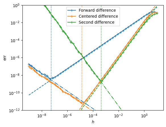
The first error term is due to truncation, while the second estimates the round-off error. Minimizing the error gives an estimate of the optimal step size:
Do It! Prove the Lagrange remainder theorem.
Prove that under suitable conditions on \(f(x)\) (state these):
and similarly for the other derivatives (assuming no round-off error). Hint: use the mean-value theorem.
Solution
A simple proof of Taylor’s theorem is due to [Cox, 1851] who considers the following quantity
Cox argues that, since \(Q_n(0) = Q_n(h) = 0\), by the mean-value theorem, \(Q'_n(x_1) = 0\) for some intermediary point \(x_1 \in (0, h)\). Continuing, since \(Q'_{n}(0) = 0\), there is another intermediary point \(x_2 \in (0, x_1)\) where \(Q''_{n}(x_2) = 0\) vanishes, and so forth until finally \(Q^{(n)}_{n}(x_{n}) = 0\) for some \(x_n \in (0, h)\). This implies
establishing the Lagrange form of the remainder in Taylor’s theorem
for some \(x^* = a+x_n \in (a, a+h)\). For this argument to hold, all \(n\) derivatives of \(f(x)\) must be continuous. It remains a simple exercise to verify that \(Q_{n}(0) = Q_{n}(h) = 0\) and that all derivatives \(Q_{n}^{(i)}(0) = 0\) for \(i < n\).
These techniques can be implemented fairly efficiently for images using
scipy.ndimage.correlate1d():
from scipy.ndimage import correlate1d
from phys_581.testing import Functions
L = 10.0
Nx = 100
h = dx = L/Nx
# Note: it is important to use proper lattice points - excluding one endpoint - if
# wrapping.
x = np.arange(Nx) * dx
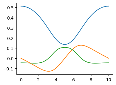
f = Functions(L=L, eta=0.5)
df = correlate1d(f(x), weights=[-1/2/dx, 0, 1/2/dx], mode='wrap')
assert np.allclose(
correlate1d(f(x), weights=[-1/2/dx, 0, 1/2/dx], mode='wrap'),
(f(x+h) - f(x-h))/2/h)
assert np.allclose(
correlate1d(f(x), weights=[0, -1/dx, 1/dx], mode='wrap'),
(f(x+h) - f(x))/h)
assert np.allclose(
correlate1d(f(x), weights=[1/dx**2, -2/dx**2, 1/dx**2], mode='wrap'),
(f(x+h) + f(x-h) - 2*f(x))/h**2)
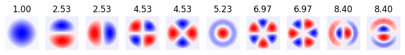
Application: Drums#
A neat application of finite differences is to estimate the normal modes of a drum.
Consider a thin 2D drum-head streched taught over a frame outlining some specified region of the \(x\)-\(y\) plane. Small-amplitude oscillations of the drum can be described by their height \(f(x,y,t)\) and will satisfy the 2D wave equation:
where \(c\) is the speed of sound in the material which will depend on the tension and mass density of the drumhead (assumed to be uniform). The solutions must satisfy the boundary condition \(f(x,y,t) = 0\) wherever the point \((x,y)\) lies on (or outside) of this region. (Dirichlet boundary conditions.)
The strategy will be to formulate a matrix representation of the laplacian \(\nabla^2\) and then look for eigenfunctions \(\nabla^2 f_n = -\frac{\omega^2_n}{c^2} f_n\). From these eigenfunctions we can form the time-dependent solutions:
where \(a_n\) are arbitrary complex coefficients.
The trick is to note that we can trivially implement Dirichlet boundary conditions by simply discarding points outside of the region that vibrates. Thus, we first form a finite difference approximation to \(\nabla^2\) on a regular grid using a tensor product of two 1-dimensional finite difference matrices, then we simply select the rows and columns that correspond to vibrating points. The resulting matrix is Hermitian, and we simply find the eigenvalues and eigenvectors which give us the normal modes and frequencies:
For more examples see Physics 571: Drums.
Warning
This trick of enforcing the boundary conditions by simply discarding lattice points outside of the zone of vibration is specific to Dirichlet boundary conditions: it depends crucially on the property that truncation is equivalent to setting the function to zero in the discarded regimes.
We will continue our exploration computing derivatives with Fourier Techniques.