Model Fitting Details#
Recall that, to fit a model \(y = f(x, \vect{a})\) that depends on \(M\) parameters \(\vect{a}\) to a collection of measurements \(\vect{y} = f(\vect{x}, \vect{a}) + \vect{e}\) where the errors \(e_{n}\) are random variables with overall PDF \(p_e(\vect{e})\), Bayes’ theorem says:
where the likelihood function is:
Least Squares
The familiar procedures of least-squares accomplishes these goals as follows. First
minimizing \(\chi^2\) express this in terms of a best-fit set of parameters \(\bar{\vect{a}}\) and a local characterization of the maximum as a quadratic form expressed in terms of a covariance matrix \(\mat{C}\).
However, to do this properly requires knowing the posterior over the full integration range (not just near the maximum), and generally results in nasty functions that cannot be done analytically. The one case in which everything has simple analytic results is if the final distribution is gaussian, but this only generically happens if both the errors and priors are gaussian and the model is linear. If the errors are small, then a linear approximation to the model may be sufficient, and
Goals of Model Fitting
The model-fitting goals discussed at the end of section 15.0.0 of [Press et al., 2007] can be expressed as
“Best fit” parameters maximize the posterior \(p(a|\vect{y})\). If the prior doesn’t depend on \(a\) (e.g. flat), then this is a maximum likelihood estimation.
Uncertainties are characterized by the shape of the posterior \(p(a|\vect{y})\).
Goodness-of-fit can be expressed through the model evidence \(p(\vect{y})\), which balances likelihood with model complexity but the issue is more complicated: see, for example, this discussion on stack overflow.
Independently Distributed Errors#
The most common formulation follows from considering flat priors (\(p(\vect{a})\) is independent of \(\vect{a}\)) and errors that are independently distributed with a common probability distribution \(N(x)\) where \(x = e_n/\sigma_n\):
I.e., the probability of simultaneously realizing all of the errors \(\vect{e}\) is the probability of realizing \(e_0\), and \(e_1\), and \(e_2\), etc.
The most common case is that of errors distributed normally with zero mean and standard deviation \(\sigma_n\):
but we can consider any distribution \(N(x)\).
Maximizing the posterior \(p(\vect{a}|\vect{y})\) is then equivalent to maximizing the likelihood, which we express as minimizing the following objective function \(F(\vect{a})\):
At the minimum \(\bar{\vect{a}}\), the objective function has zero gradient, and hence is approximately quadratic, described by the Hessian matrix \(\mat{H}\):
If the errors are normal (gaussian), then \(\rho(x) = -\ln N(x) = x^2/2\), and we recover the familiar approach of minimizing \(\chi^2\), the sum of the square of the residuals:
In this case, the Hessian matrix \(\mat{H} = \mat{C}^{-1} = \mat{\Sigma}^{-1}\) is exactly the inverse of the covariance matrix \(\mat{C}\), and the posterior distribution is approximately a multivariate normal distribution with mean \(\bar{\vect{a}}\) and covariance matrix \(\mat{C} = \mat{\Sigma} = \mat{H}^{-1}\) after normalizing
where there are \(M\) parameters \(\vect{a} = (a_0, a_1, \dots, a_{M-1})\).
Poisson Distribution (Incomplete)
Poisson Distribution (Incomplete)
As another example, supposed your data \(y_n\) comes from counting (e.g. photons on a
detector). In this case, the errors are probably more appropriately described by a
Poisson distribution. For example, supposed we have a photo-detector that measures
photons at a location \(x\) with spatial probability distribution \(n(x) =
\abs{\psi(x)}^2\) which is some wavefunction that we want to model.
The detectors will count photons at some rate average rate \(r = \alpha n(x)\d{x}\) where
\(\d{x}\) is the pixel size and \(\alpha\) is some capture rate (photons per unit time)
which is a property of the detector. If the detector is on for time \(t\), then the
average number of photons measured at \(x\) will be \(\lambda = rt\) and our data point will
be \(y = n(x) = rt/\alpha t \d{x}\).
The probability of measuring \(k\) photons in the time \(t\) is:
Parameter Uncertainties (Covariance)#
A complete characterization of the posterior \(p(\vect{a}|\vect{y})\) is usually provided through a large set of sample data \(\{\vect{a}_n\}\) sampled with the appropriate probability from this distribution. The goal of methods like Markov chain Monte Carlo (MCMC) is to generate such a distribution.
Alternatively, the posterior might be known analytically. This is the case if both the prior and likelihood are multivariate normal distributions (i.e. if the model is linear and the errors are normally distributed):
Marginal Distributions#
Once one obtains the posterior distribution \(p(\vect{a}|\vect{y})\), one needs to communicate this. The first thing one might do is to look at the uniform probability distribution for each parameter:
This gives us an idea about how the parameter \(a_{i}\) is distributed. In particular, one can plot these distributions using a histogram, or one can present numerical values of various statistical features like:
the mean, median, or mode, which act as a description of the “best fit” parameter values;
the standard deviation, which acts as a description of the uncertanties; and
the skewness, kurtosis, etc. which characterize how different the distribution is from a [normal distrbution] (along with the differences between the mean, median, and mode).
Pairwise distributions
can also be easily visualized through a corner plot plot.
The Gaussian Case#
If your posterior is well approximated by a multivariate normal distribution, then one can analytically compute the marginal distributions. The result is simply obtained by taking the appropriate columns and rows of the covariance matrix \(\mat{C}\):
This generalizes to any set of parameters, but see the note below about how to interpret these regions.
Confidence Levels#
When considering a marginal distribution of \(\nu\) variables constructed this way, you should determine your confidence region by using the corresponding \(\chi^2\) distribution with \(\nu\) degrees of freedom \(P_{\chi^2, \nu}(\chi^2)\). Specifically, to find the confidence regions containing fraction \(p\) of the total samples over \(\nu\) variables, you should consider the region
with \(p_{1\sigma}=68.27\%\) for the \(1\sigma\) confidence level, \(p_{2\sigma}=84.27\%\), \(p_{3\sigma} = 91.67\%\), \(p_{4\sigma} = 95.45\%\), etc.
The value \(\chi^2_p\) can be computed with the scipy.stats.rv_continuous.ppf()
method of the scipy.stats.chi2 distribution. For \(\nu=1\) we have simply
\(\chi^2_p = n\) for the \(n\sigma\) confidence level, but this differs for \(\nu > 1\). See
Confidence Regions for details.
Important
There are several important caveats here:
This only makes sense if your model is a good fit (i.e. \(Q > 0.001\)). If your model is not good, you can pretend like you do not know the distribution of your errors, and scale the uncertainties by an overall factor to make \(\chi^2_r = 1\). This corresponds to scaling:
(2)#\[\begin{gather} \sigma_n \rightarrow \sigma_n \sqrt{\chi^2_r}, \qquad \mat{C} \rightarrow \chi^2_r\mat{C}. \end{gather}\]Another option: if your experimental errors are independent and identically distributed (iid), you can use the bootstrap method discussed in section 15.6.2 of [Press et al., 2007] to use the data itself to estimate the errors.
If your distribution is not gaussian, then the relationship between the contours \(\chi^2_p\) and the confidence level \(p\) will likely not be given by the chi square distribution \(P_{\chi^2, \nu}(\chi^2)\). If the errors are small, one can still use this approach as the posterior distribution will still be approximately quadratic close to the maximum at \(\vect{a} = \bar{\vect{a}}\):
\[\begin{gather*} -2\ln \frac{p(\vect{a}|\vect{y})}{p(\bar{\vect{a}}|\vect{y})} \approx \delta\vect{a}^T \mat{C}^{-1} \delta\vect{a}, \qquad \delta \vect{a}^T\mat{C}^{-1}\delta \vect{a} \leq \chi^2_p. \end{gather*}\]Hence, one can still approximate the confidence region from the levels of constant \(\chi^2_p\), but the relationship between this and \(p\) must now be determined by a simple Monte Carlo calculation as discussed in section 15.6.1 of [Press et al., 2007].
If you want to explore a smaller set of \(\tilde{\nu} < \nu\) parameters, you can integrate the posterior distribution over the \(\nu - \tilde{\nu}\) “nuisance” parameters by just keeping the corresponding rows and columns of \(\mat{C}\) in a new smaller matrix \(\tilde{\mat{C}}\) as discussed above for the cases \(\tilde{nu} = 1\) and \(\tilde{nu} = 2\). This corresponds to minimizing over the nuisance parameters. Note: do not extract the rows and columns of \(\mat{C}^{-1}\) which would correspond to holding the nuisance parameters fixed, which is almost certainly not what you want to do.
Once you have done this, you can explore the contour in this marginal distribution corresponding to
\[\begin{gather*} \Delta \tilde{\chi}^2(\tilde{\vect{a}}) \approx \delta\tilde{\vect{a}}^T \tilde{\mat{C}}^{-1} \delta\tilde{\vect{a}} < \chi^2_{p} \end{gather*}\]where you must determine \(\chi^2_{p}\) from the inverse (CDF) for the chi squared distribution with \(\tilde{\nu}\) degrees of freedom if your posterior is gaussian, or using Monte Carlo.
The Geometry of Data Fitting#
Data fitting can be visualized geometrically as follows. Consider \(N\) data points \(\vect{y} = (y_{0}, y_{1}, \dots, y_{N-1})\) as a vector \(\vect{y} \in \mathbb{R}^{N}\). A model with \(M\) parameters \(\vect{a}\) can now be though of as an \(M\)-dimensional surface in \(\mathbb{R}^{N}\) as defined by the set of points \(\vect{f}(\vect{a})\).
Example: Three Points#
The geometry of fitting a two-parameter curve \(y_n = f(x_n, \vect{a})\) to three data points \(\vect{y}\) can be visualized in 3D. Here we demonstrate two models, one linear, and another exponential.
The linear model (middle green) gives a plane in the 3D space of points \(\vect{y}\), while the exponential model (right, red) gives a curved surface with a singular point where \(a_0=0\). The data \(\vect{y}\) is the orange point. The best-fit problem reduces to finding the point on these surfaces which is closest to the data in terms of of the \(L_2\) norm \(\norm{\vect{y}}_2 \sqrt{\chi^2}\). These solutions ate noted by black crosses. In this picture, the vector from the best fit point to the data (orange line) is normal to the surface.
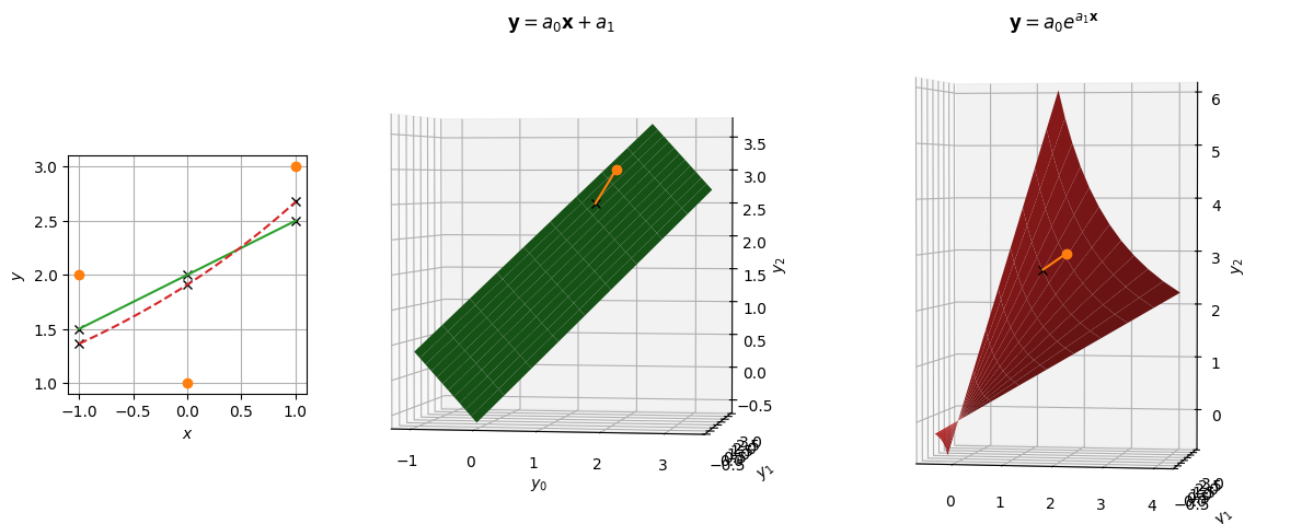
The geometry is the same with other norms, but the notion of distance and angles can change. This same picture can be used with unequal errors by first scaling the data and functions \(y_n \rightarrow y_n/\sigma_n\), \(f(x, \vect{a}) \rightarrow f(x,\vect{a})/\sigma(x_n)\) where \(\sigma(x_n) = \sigma_n\) is an appropriate function. These factors of \(\sigma_n\) can also just be absorbed into a redefined metric.
Complete Example#
Here we work through a complete example of a single parameter model \(y_n = a + e_n\) with independent gaussian error distributions \(p_n(e_n)\) with zero mean (unbiased) and variance \(\sigma_n^2\). This simplifies things, because the product of gaussian distributions is gaussian:
We start with gaussian prior \(p(a)\) with mean \(a_p\) and variance \(\sigma_p^2\). After a measurement with value \(y_0\), our posterior is:
, after several measurements \(y_0\), \(y_1\), and \(y_2\), we have posteriors
Note that the order in which we include the measurements makes no difference, as expected from the final form \(p(a|\vect{y}) \propto p_e(\vect{y}-\vect{e})p(a)\).
Consider a single measurement, but now with two error estimates \(p_0(e_0)\) and an underestimated error \(\tilde{p}_0(e_0) = \lambda p_0(\lambda e_0)\)
These are not the same. Consider a flat prior and normally distributed errors with correct \(\sigma\) and incorrect \(\tilde{\sigma} = \sigma / \lambda\):