Globally Convergent Newton’s Method#
For finding solutions to non-linear equations \(f(x) = 0\), Newton’s method can converge extremely quickly, roughly doubling the number of digits each step.
However, if the initial state is poorly chosen, it can converge very slowly, or even diverge. By carefully choosing both the form of \(f(x) = 0\) and the initial guess, one can often design an algorithm that will converge for all initial states with a few iterations at most. This is an art rather than a science. Here we show some examples.
Polynomial Inversion#
An example came up in Random Variables when trying to invert the cumulative
distribution function \(C_Z(z) = (-x^3 + 3x + 2)/4\) corresponding to the Thomas-Fermi PDF
\(P_Z(z) = 3(1-z^2)/4\). The roots of a polynomial can be found quite efficiently with
numpy.roots(), but this returns all 3 roots, and in this case, we want a
specific one.
First we plot the function, and note that it is very well approximated by:
z = np.linspace(-1, 1)
P = np.array([-1, 0, 3, 2])/4

fig, ax = plt.subplots()
ax.plot(z, np.polyval(P, z), label=r"$C_Z(z)$")
ax.plot(z, (1+np.sin(np.pi*z/2))/2, ":", label=r"$[1+\sin(\pi z/2)]/2$")
ax.legend()
ax.set(xlabel="$z$", ylabel="$C_Z(z)$");
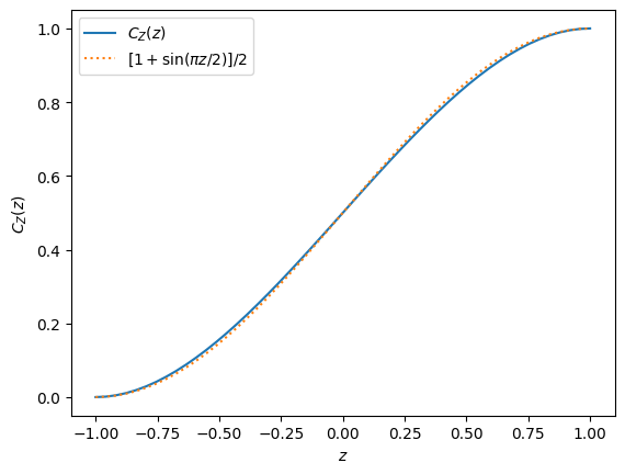
This suggests a globally convergent strategy for solving \(x = C_Z(z)\):
To check this, we see how many iterations it takes to reach a specified tolerance, and then plot this over the range of inputs:
P = np.array([-1, 0, 3, 2])/4
dP = np.polyder(P)

def C_Z(z):
    return np.polyval(P, z)

def C_Z_inv(x, n):
    """Perform `n` steps of Newton's method to invert `x=C_Z(z)`"""
    z = 2/np.pi * np.arcsin(2*x-1)
    for _n in range(n):
        z -= (np.polyval(P, z) - x) / np.polyval(dP, z)
    return z

# Skip endpoints where denominator will be zero
z = np.linspace(-1, 1, 1000)[1:-1]
x = C_Z(z)

fig, ax = plt.subplots()
for n in [0, 1, 2, 3, 4]:
    ax.semilogy(x, abs(C_Z_inv(x, n=n) - z), label=f"n={n}")
ax.legend()
ax.set(xlabel="$x$", ylabel="$|C_Z^{-1}(x)-z|$");
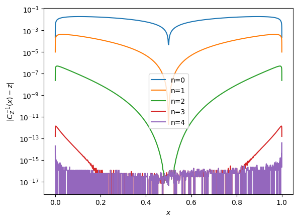
This shows that we achieve machine precision with 3 iterations if \(x \in [0.2, 0.8]\) and in 4 iterations everywhere else, except near the boundaries. Let’s look a little more closely there (noting that the behavior is symmetric):
# Skip endpoints where denominator will be zero
z = -1 + 10**(np.linspace(-8, 0, 100))
x = C_Z(z)

fig, ax = plt.subplots()
for n in [0, 1, 2, 3, 4]:
    ax.loglog(x, abs(C_Z_inv(x, n=n) - z), label=f"n={n}")
ax.legend()
ax.set(xlabel="$x$", ylabel="$|C_Z^{-1}(x)-z|$");
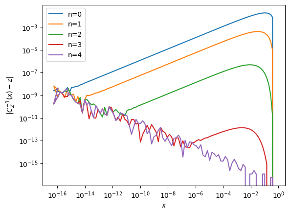
The fluctuations here seem to indicate that the issue at the boundary is actually due to roundoff error, so we have are finished with the following:
def C_Z(z, P=[-1, 0, 3, 2]):
    return np.polyval(P, z)/4

def C_Z_inv(x, P=[-1, 0, 3, 2], dP=[-3, 0, 3]):
    """Invert `x=C_Z(z)`"""
    z = 2/np.pi * np.arcsin(2*x-1)
    for _n in range(4):
        z -= (np.polyval(P, z) - 4*x) / (np.polyval(dP, z) + 1e-32)
    return z

x = np.linspace(0, 1, 1000)
z = C_Z_inv(x)
assert np.allclose(C_Z(z), x, atol=1e-15)
Lambert W Function#
Here we consider the example from Assignment 1: Recursion and Invariants, computing the \(k=0\) branch of the Lambert W function \(W_0(z)\) which inverts \(z=we^w\). We want an efficient algorithm that works for.
Copilot
Here is what MS Copilot gives:
Write a function in Python that efficiently computes the k=0 branch of the Lambert W function.
from scipy.special import lambertw

def lambert_w_k0(x):
    return lambertw(x, k=0).real  # returns the real part for real x
This is a good solution since the function exists in SciPy, but we want one we can understand. This algorithm uses Halley’s method, which generalizes Newton’s method to Padé approximants:
import math

def lambert_w_k0(x, max_iter=100, tol=1e-12):
    if x == 0:
        return 0.0
    if x < -1 / math.e:
        raise ValueError("Lambert W function not defined for x < -1/e on the principal branch.")

    # Initial guess
    w = math.log1p(x) if x < 1 else math.log(x) - math.log(math.log(x))

    for _ in range(max_iter):
        ew = math.exp(w)
        wew = w * ew
        diff = wew - x
        denom = ew * (w + 1) - (w + 2) * diff / (2 * w + 2)
        w_new = w - diff / denom
        if abs(w_new - w) < tol:
            return w_new
        w = w_new

    return w  # Return after max_iter if not converged
Test-Driven Development#
We first want to make sure that any function we give works, so lets write some tests. The domain is \(z \in [-1/e, \infty)\), which we can sample with
Nx = 100
x = np.linspace(0, 1, Nx)[1:-1]
z = 1/x - 1 - np.exp(-1)  # Sample points from -e to infinity

# Don't sit exactly on -1 as roundoff errors can push this off the branch.
w = np.linspace(-1+1e-9, 1, Nx)
z = w * np.exp(w)

def test1(W, z=z):
    w = W(z)
    assert np.allclose(w * np.exp(w), z)
    assert np.allclose(np.log(abs(w)) + w, np.log(abs(z)), atol=1e-15, rtol=1e-15)

# Check that the implemention in SciPy works.
import scipy as sp
test1(sp.special.lambertw)
A First Attempt#
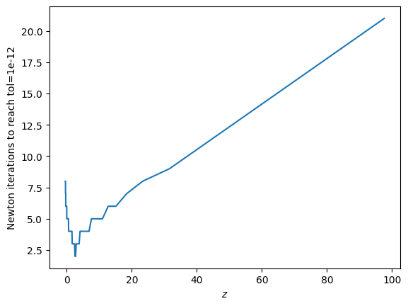
Let’s simply apply Newton’s method with an initial guess of \(w=1\):
def newton_iter_1(w, z):
    """Perform one step of Newton's iteration."""
    f = w*np.exp(w) - z
    df = (1+w)*np.exp(w)
    return w - f/df
    return (w**2 + z*np.exp(-w))/(1+w)  # More efficient, but risky

def get_w0(z):
    """Get an initial guess."""
    return 1 + 0*z

@np.vectorize
def count(get_w0, iter, z=z, maxiter=100, tol=1e-12):
    w = get_w0(z)
    for n in range(maxiter):
        w = iter(w, z=z)
        if abs(np.log(abs(w)) + w - np.log(abs(z))) < tol:
            break
    if n == maxiter - 1:
        n = -1
    return n


tol = 1e-12
Nx = 100
x = np.linspace(0, 1, Nx)[1:-1]
z = 1/x - 1 - np.exp(-1)  # Sample points from -e to infinity
Niter = count(get_w0=get_w0, iter=newton_iter_1, z=z, tol=tol)
fig, ax = plt.subplots()
ax.plot(z, Niter)
ax.set(xlabel="$z$", ylabel=f"Newton iterations to reach {tol=}");
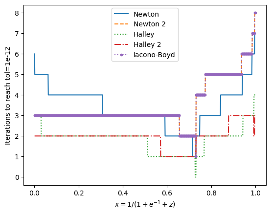
For comparison, we consider two other iterations. First a Newton iteration based on the log of the equation:
The second is based on Halley’s method:
which we apply to both formulations.
def newton_iter_2(w, z):
    """Perform one step of Newton's iteration."""
    f = np.log(abs(w)) + w - np.log(abs(z))
    df = 1/w + 1
    return w - f/df
    return (w**2 + z*np.exp(-w))/(1+w)  # More efficient, but risky

def halley_iter_1(w, z):
    """Perform one step of Halley's iteration."""
    f = w*np.exp(w) - z
    df = (1+w)*np.exp(w)
    ddf = (2+w)*np.exp(w)
    return w - f*df/(df**2 - f*ddf/2)

def halley_iter_2(w, z):
    """Perform one step of Halley's iteration."""
    f = np.log(abs(w)) + w - np.log(abs(z))
    df = 1/w + 1
    ddf = -1/w**2
    return w - f*df/(df**2 - f*ddf/2)

def lacono_boyd_1(w, z):
    return w/(1+w)*(1 + np.log(abs(z/w)))

fig, ax = plt.subplots()
for iter, fmt, label in [(newton_iter_1, '-', "Newton"),
                         (newton_iter_2, '--', "Newton 2"),
                         (halley_iter_1, ':', "Halley"),
                         (halley_iter_2, '-.', "Halley 2"),
                         (lacono_boyd_1, '.:', "lacono-Boyd")]:
    Niter = count(get_w0=get_w0, iter=iter, z=z, tol=tol)
    ax.plot(x, Niter, fmt, label=label)
ax.set(xlabel="$x = 1/(1+e^{-1} + z)$", ylabel=f"Iterations to reach {tol=}")
ax.legend();
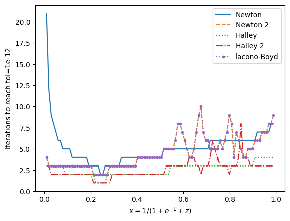
Halley’s method works remarkably well here, but Newton’s method applied to an appropriately transformed function also works very well.
The next step is to try to improve the initial guess.
def get_w1(z):
    return np.where(z < 0, z*np.exp(-1), np.log(abs(z)+1))

tol = 1e-12
Nx = 1000
x = np.linspace(0, 1, Nx)[1:-1]
z = 1/x - 1 - np.exp(-1)  # Sample points from -e to infinity

fig, ax = plt.subplots()
for iter, fmt, label in [(newton_iter_1, '-', "Newton"),
                         (newton_iter_2, '--', "Newton 2"),
                         (halley_iter_1, ':', "Halley"),
                         (halley_iter_2, '-.', "Halley 2"),
                         (lacono_boyd_1, '.:', "lacono-Boyd")]:
    Niter = count(get_w0=get_w1, iter=iter, z=z, tol=tol)
    ax.plot(x, Niter, fmt, label=label)
ax.set(xlabel="$x = 1/(1+e^{-1} + z)$", ylabel=f"Iterations to reach {tol=}")
ax.legend();