Show code cell content

Hide code cell content

import mmf_setup

mmf_setup.nbinit()
import logging

logging.getLogger("matplotlib").setLevel(logging.CRITICAL)
%matplotlib inline
import numpy as np, matplotlib.pyplot as plt

$\newcommand{\vect}[1]{\mathbf{#1}} \newcommand{\uvect}[1]{\hat{#1}} \newcommand{\abs}[1]{\lvert#1\rvert} \newcommand{\norm}[1]{\lVert#1\rVert} \newcommand{\I}{\mathrm{i}} \newcommand{\ket}[1]{\left|#1\right\rangle} \newcommand{\bra}[1]{\left\langle#1\right|} \newcommand{\braket}[1]{\langle#1\rangle} \newcommand{\Braket}[1]{\left\langle#1\right\rangle} \newcommand{\op}[1]{\mathbf{#1}} \newcommand{\mat}[1]{\mathbf{#1}} \newcommand{\d}{\mathrm{d}} \newcommand{\D}[1]{\mathcal{D}[#1]\;} \newcommand{\pdiff}[3][]{\frac{\partial^{#1} #2}{\partial {#3}^{#1}}} \newcommand{\diff}[3][]{\frac{\d^{#1} #2}{\d {#3}^{#1}}} \newcommand{\ddiff}[3][]{\frac{\delta^{#1} #2}{\delta {#3}^{#1}}} \newcommand{\floor}[1]{\left\lfloor#1\right\rfloor} \newcommand{\ceil}[1]{\left\lceil#1\right\rceil} % The following allows KaTeX to render these for significantly improved % performance on CoCalc. \newcommand{\DeclareMathOperator}[2]{\newcommand{#1}{#2}} \DeclareMathOperator{\Tr}{Tr} \DeclareMathOperator{\erf}{erf} \DeclareMathOperator{\erfi}{erfi} \DeclareMathOperator{\sech}{sech} \DeclareMathOperator{\sn}{sn} \DeclareMathOperator{\cn}{cn} \DeclareMathOperator{\dn}{dn} \DeclareMathOperator{\sgn}{sgn} \DeclareMathOperator{\order}{O} \DeclareMathOperator{\diag}{diag} % \newcommand{\mylabel}[1]{\label{#1}\tag{#1}} \newcommand{\degree}{\circ}$

This cell adds /home/docs/checkouts/readthedocs.org/user_builds/wsu-phys-581-computation/checkouts/latest/src to your path, and contains some definitions for equations and some CSS for styling the notebook. If things look a bit strange, please try the following:

• Choose "Trust Notebook" from the "File" menu.
• Re-execute this cell.
• Reload the notebook.

Quantum Mechanics in 1D

The central object in non-relativistic quantum mechanics for a single particle in one dimension is the wavefunction \(\psi(x, t)\), which satisfies the Schrödinger equation:

\[\begin{gather*} \I\hbar \pdiff{\psi(x, t)}{t} = \frac{-\hbar^2}{2m}\pdiff[2]{\psi(x, t)}{x} + V(x)\psi(x, t). \end{gather*}\]

Although this is a partial differential equation, one typically deals with independent boundary conditions in space and time, so one can view this as first-order ODE in time once a suitable basis found:

\[\begin{gather*} \I\hbar \diff{}{t}\ket{\psi(t)} = \op{H}\ket{\psi(t)} \end{gather*}\]

where \(\op{H}\) is some linear operator called the Hamiltonian, which will become a matrix once expressed in some basis. I.e. consider a set of orthonormal basis vectors \(\ket{j}\):

\[\begin{gather*} \braket{i|k} = \delta_{ij}, \qquad \sum_{j} \ket{j}\bra{j} = \mat{1}. \end{gather*}\]

Acting on this equation with \(\bra{i}\) and inserting the identity \(\mat{1} = \sum_{j} \ket{j}\bra{j}\) we obtain the matrix equation:

\[\begin{gather*} \I\hbar \diff{}{t}\overbrace{\braket{i|\psi(t)}}^{\psi_i(t)} = \sum_{j}\overbrace{\braket{i|\op{H}|j}}^{H_{ij}}\overbrace{\braket{j|\psi(t)}}^{\psi_j(t)}. \end{gather*}\]

Thus, once we figure out an appropriate basis, and express the Hamiltonian operator as a matrix in this base, we can implement the time-dependent Schrödinger equation using the techniques discussed in Assignment 2: IVPs and ODEs.

Fourier Bases

The best choice of basis depends on the nature of the problem, and the boundary conditions. If the potential \(V(x)\) is smooth and one can work with periodic boundary conditions, then Fourier bases can work extremely well. I.e. if the potential is an analytic function, then Fourier bases can give exponential convergence in the lattice spacing. They are also extremely convenient and performant given the availability of the [FFT] on both CPU and GPU architectures. Here we present a quick summary of their properties, for details see Fourier Basis.

When not to use a Fourier basis (click for details):

Non-periodic boundary conditions

If your potential is analytic, but your boundary conditions are not periodic, consider if an expanded domain might help. For example, Dirichlet/Neumann boundary conditions can be imposed by doubling the domain and stitching together flipped versions of the wavefunction so that the symmetry imposes the appropriate boundary conditions. One might also be able to pad the basis with enough points so that the wavefunction vanishes at the boundaries. We will do this to solve for the Harmonic oscillator.

Alternatively, consider using a Chebyshev basis. This may have some issues, e.g. one can not use the FFT, and the Hamiltonian may not be hermitian. Exponential convergence may mean you can keep the basis size small enough that these technical issues are not practical problems.

Non-analytic potentials

If your potential is non-analytic, then you will not have exponential convergence. This may be okay – finite differences will not have exponential convergence either – and the efficiency of the FFT might still make this the method of choice.

Sometimes, the non-analyticity can be dealt with specifically by an appropriate choice of basis. This is how DVR bases are constructed, for example, restoring exponential convergence. See [Littlejohn et al., 2002] and references therein for more details.

In computer science, and some physics texts, the factor of \(2\pi\) is split so that the transforms become more symmetric:

\[\begin{align*} \newcommand{\k}{\smash{\tilde{k}}} \newcommand{\p}{\smash{\tilde{p}}} \tilde{\psi}_k &= \int\d{x} \frac{e^{-\I k x}}{\sqrt{2\pi}}\psi(x),\\ \psi(x) &= \int\d{k} \frac{e^{\I k x}}{\sqrt{2\pi}}\tilde{\psi}_k,\\ \braket{x|\k} &= \frac{e^{\I k x}}{\sqrt{2\pi}}. \end{align*}\]

This effected from our notation by taking \(\ket{\k} \rightarrow \ket{\k}/\sqrt{2\pi}\):

\[\begin{align*} \op{1} &= \int \d{x}\ket{x}\bra{x} \\ &= \int \d{k}\ket{\k}\bra{\k}. \end{align*}\]

We prefer to keep all factors of \(2\pi\) in one place: in the measure \(\d{k}/2\pi\).

We shall use the following basis and normalization (common in physics) for the continuum, then specialize to the lattice and periodic box. The key relationship comes from:

\[\begin{gather*} \int_{-\infty}^{\infty}\frac{\d{k}}{2\pi} e^{\I k (x-y)} = \delta(x-y). \end{gather*}\]

A normalization common in particle physics is:

\[\begin{gather*} \op{1} = \int \d{x} \ket{x}\bra{x} = \int\frac{\d{k}}{2\pi}\ket{\k}\bra{\k}, \qquad \braket{x|\k} = e^{\I k x}. \end{gather*}\]

Note

Here we use late-alphabet variables \(x\), \(y\), \(z\) for position space, and mid-alphabet variables \(k\), \(l\) for the angular wavenumber with momenta \(p\) and \(q\) including a factor of \(\hbar\): \(p = \hbar k\) etc. In many cases, we will take units so that \(\hbar = 1\), in which case we may also use the variables \(p\) and \(q\) to denote momentum-space variables. Here, for clarity, we will try to include a tilde, i.e. \(\ket{\k}\), for momentum-space basis elements, but this is often dropped in the literature.

The Fourier transform will be denoted with a subscript \(\tilde{\psi}_k\) whereas positions will appear as a wavefunction \(\psi(x)\). This represents the usual approach of starting with quantum mechanics in terms of wavefunctions \(\psi(x)\), then later, expressing these in a basis with \(\tilde{\psi}_k\) being the “coefficients” in some basis \(f_k(x)\), which becomes the inverse Fourier transform in the continuum limit:

\[\begin{gather*} \psi(x) = \sum_k \tilde{\psi}_k f_k(x) \rightarrow \int \frac{\d{k}}{2\pi} \tilde{\psi}_k e^{\I k x} \end{gather*}\]

From these, it follows that

\[\begin{gather*} \braket{x|y} = \delta(x-y), \qquad \braket{\p|\k} = (2\pi)\delta(p-k). \end{gather*}\]

We can use this basis to express a wavefunction \(\psi(x) = \braket{x|\psi}\) in position space, or in momentum space \(\tilde{\psi}_k = \braket{\k|\psi}\). The Fourier transform follows from the change of bases, which we implement by inserting the identity \(\op{1}\) in the appropriate form. I.e.

\[\begin{gather*} \braket{\k|\psi} = \braket{\k|\op{1}|\psi} = \int \d{x} \braket{\k|x}\braket{x|\psi} = \int \d{x} e^{-\I k x}\psi(x),\\ \braket{x|\psi} = \braket{x|\op{1}|\psi} = \int \frac{\d{k}}{2\pi} \braket{x|\k}\braket{\k|\psi} = \int \frac{\d{k}}{2\pi} e^{\I k x}\tilde{\psi}_k. \end{gather*}\]

Restricting our domain to periodic functions in a box of length \(L\) with \(x\in [0, L)\), we find that the wavenumbers become quantized with integer \(m\):

\[\begin{gather*} e^{\I k_m (x+L)} = e^{\I k_m x} \implies k_m = \frac{2\pi m}{L}. \end{gather*}\]

If we furthermore restrict ourselves to a finite range of \(m \in \{0, 1, \dots, N-1\}\), then we can represent the span of this basis by the Nyquist–Shannon sampling theorem, evaluating the function at \(N\) equally spaced points with spacing \(\Delta x = L/N\). Once we do this, we cannot tell the difference between \(k_{m+N}\) and \(k_{m}\) – this is called aliasing – so we instead consider wavenumbers from \(m\in \{-\floor{N/2}, -\floor{N/2}+1, \dots, \floor{(N-1)/2}\}\). (The maximum point is \(N/2 - 1\) if \(N\) is even, or \((N-1)/2\) if \(N\) is odd.)

Note

For numerical purposes, the basis vectors are order \(m \in [0, 1, \dots, \floor{(N-1)/2}, -\floor{N/2}, -\floor{N/2}+1, \dots, -1]\), which can be duplicated by the following code using integer division // and the mod operation %:

n = np.arange(N)
m = (n + N//2) % N - N//2

Thus, we have a finite basis, representing the wavefunction \(\psi(x_n)\) as a vector of values by evaluating on the equally spaced abscissa \(x_n \in [0, L)\), and expressing this as a finite Fourier series in terms of the discrete wavevectors \(k_m\):

\[\begin{gather*} x_n = n \overbrace{\frac{L}{N}}^{\d{x}}, \qquad k_{m} = \overbrace{\frac{2\pi}{L}}^{\d{k}} m. \end{gather*}\]

To connect with the continuum formula, we use the Riemann sums:

\[\begin{align*} \overbrace{\d{x}}^{L/n}\sum_{n} &\leftrightarrow \int_0^{L} \d{x}, \\ \overbrace{\d{k}}^{2\pi/L}\sum_{m} &\leftrightarrow \int_{-k_{\max}/2}^{k_{\max}/2} \d{k}, \\ \frac{1}{N}\sum_{m} &\leftrightarrow \int_{-k_{\max}/2}^{k_{\max}/2} \frac{\d{k}}{2\pi}. \end{align*}\]

We normalize the basis functions and overlaps so that all Dirac delta-functions become Kronecker deltas:

\[\begin{gather*} \mat{1} = \sum_{n} \ket{x_n}\bra{x_n} = \sum_{m} \ket{\k_m}\bra{\k_m},\\ \braket{x_n|\k_m} = \frac{1}{\sqrt{N}} e^{\I k_m x_n}, \qquad [\mat{U}]_{nm} = \braket{x_m|x_n} = \braket{\k_m|\k_n} = \delta_{mn}. \end{gather*}\]

The Fourier transform is effected by the matrix \(\sqrt{N} \mat{U}^\dagger\) and the inverse is effected by \(\mat{U}/\sqrt{N}\). (The normalization is included this way for performance.)

Derivatives are trivially computed in the wavenumber basis using the representations of the momentum operator::

\[\begin{gather*} \braket{\k_m|\op{p}|\k_n} = -\I\hbar k_n \delta_{mn}, \qquad \braket{\k_m|\op{p}^2|\k_n} = -\hbar^2k_n^2\delta_{mn},\\ \pdiff{}{x} \equiv \frac{\op{p}}{-\I\hbar}, \qquad \pdiff[2]{}{x} \equiv \frac{\op{p}}{-\hbar^2}. \end{gather*}\]

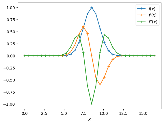
Here we check this numerically using a basis of length \(L\) and a Gaussian that falls off sufficiently fast:

\[\begin{gather*} f(x) = e^{-(x-x_0)^2/2}, \qquad f'(x) = -(x-x_0)f(x), \qquad f''(x) = \bigl((x- x_0)^2 - 1\bigr)f(x),\\ \int f(x) \d{x} = \sqrt{2\pi}. \end{gather*}\]

L = 17.0
def f_x(x, d=0):
    x0 = L/2
    f = np.exp(-(x-x0)**2/2)
    if d == 0:
        return f
    elif d == 1:
        return -(x-x0)*f
    elif d == 2:
        return ((x-x0)**2 - 1)*f


def f_k(k):
    return np.exp(-k**2/2)


for N in [33, 32]:
    dx = L/N
    dk = 2*np.pi / L
    n = np.arange(N)
    xs = dx * n
    ks = 2 * np.pi * np.fft.fftfreq(N, dx)
    
    # The columns of this matrix are the basis vectors normalized numerically
    U = np.exp(1j*ks[np.newaxis, :]*xs[:, np.newaxis]) / np.sqrt(N)

    # Check that the basis is orthonormal by ensuring that U is unitary.
    assert np.allclose(U.T.conj() @ U, np.eye(N))
    
    # Check that our formula in the sidebar is correct
    _m = (n + N//2) % N - N//2
    assert np.allclose(ks, 2 * np.pi * _m /L)
    
    # Integrate the gaussian using the basis
    f_xs = f_x(xs)
    f_ks = f_k(ks)
    dk = 2 * np.pi / L
    assert np.allclose(sum(f_xs) * dx, np.sqrt(2*np.pi))
    assert np.allclose(sum(f_ks) * dk, np.sqrt(2*np.pi))
    
    # Check the FFT normalizations claimed in the text.
    assert np.allclose(np.fft.fft(f_xs), U.T.conj() @ f_xs * np.sqrt(N))
    assert np.allclose(np.fft.ifft(f_ks), U @ f_ks / np.sqrt(N))
    
    # Check derivatives
    D1 = 1j*ks   # In wavevector basis
    if N % 2 == 0:
        # With even basis, the middle momentum is unpaired.
        # We zero this out.
        D1[N//2] = 0
    D2 = -ks**2
    assert np.allclose(f_x(xs, d=1), np.fft.ifft(D1 * np.fft.fft(f_xs)))
    assert np.allclose(f_x(xs, d=2), np.fft.ifft(D2 * np.fft.fft(f_xs)))
    
fig, ax = plt.subplots()
ax.plot(xs, f_x(xs), "+-", label="$f(x)$")
ax.plot(xs, f_x(xs, d=1), "+-", label="$f'(x)$")
ax.plot(xs, f_x(xs, d=2), "+-", label="$f''(x)$")
ax.legend()
ax.set(xlabel="$x$");

Galilean Transformation.

We now check the form of a Galilean transformation. We will implement this with

\[\begin{gather*} x_0(t) = \frac{at^2]{2}, \qquad \dot{x}_0(t) = at, \qquad \ddot{x}_0(t) = a, \\ \int_{0}^{t}\dot{x}_0^2\d{t} = \frac{a^2t^3}{3}. \end{gather*}\]

from scipy.linalg import expm

hbar = 1.2
m = 1.3
a = 0.6
t = 0.2

I = np.eye(N)
P = U @ np.diag(hbar * ks) @ U.T.conj()
X = np.diag(xs)

V = f_x
V_x = V(xs)

def x0(t, d=0):
    if d == 0:
        return a*t**2/2
    elif d == 1:
        return a*t
    elif d == 2:
        return a
    else:
        # Integral of v^2
        return a**2*t**3/3

def x0(t, d=0):
    if d == 0:
        return a*t**3/3
    elif d == 1:
        return a*t**2
    elif d == 2:
        return 2*a*t
    else:
        # Integral of v^2
        return a**2*t**5/5

def G1(t=t):
    return expm(-1j*v*(m*X - P*t)/hbar)

def G2(t=t):
    return (np.exp(1j/hbar * (m*x0(t, d=None) / 2)) * I
            @ expm(-1j/hbar * (m*x0(t, d=1)) * X) 
            @ expm(1j/hbar * x0(t, d=0) * P)
            )

h = 1e-8
dG2 = (G2(t+h) - G2(t-h))/2/h

a_ = x0(t, d=1)*P
b_ = - m*x0(t, d=2)*(X - x0(t)*I)
c_ = m/2*x0(t, d=1)**2 * I

A = -1j*hbar * G2(t).conj().T @ dG2
B = x0(t, d=1)*P - m*x0(t, d=2)*(X - x0(t)*I) + m/2*x0(t, d=1)**2 * I
C = x0(t, d=1)*P - m*x0(t, d=2)*X + m/2*x0(t, d=1)**2 * I

assert np.allclose(A @ V_x, B @ V_x)

H0 = (P@P)/2/m + np.diag(V(xs))

H1 = (P@P)/2/m + np.diag(V(xs))

G.T.conj() @ H0 @ G

---------------------------------------------------------------------------
NameError                                 Traceback (most recent call last)
Cell In[3], line 63
     59 H0 = (P@P)/2/m + np.diag(V(xs))
     61 H1 = (P@P)/2/m + np.diag(V(xs))
---> 63 G.T.conj() @ H0 @ G

NameError: name 'G' is not defined