import mmf_setup;mmf_setup.nbinit()
import logging;logging.getLogger('matplotlib').setLevel(logging.CRITICAL)
This cell adds /home/docs/checkouts/readthedocs.org/user_builds/wsu-phys-581-computation/checkouts/latest/src to your path, and contains some definitions for equations and some CSS for styling the notebook. If things look a bit strange, please try the following:
- Choose "Trust Notebook" from the "File" menu.
- Re-execute this cell.
- Reload the notebook.
Assignment 2: IVPs and ODEs#
This assignment deals with numerically solving initial value problems (IVPs) for ordinary differential equations (ODEs) such as might arise in classical and quantum mechanics.
Finite Differences#
Test the function phys_581.assignment_2.solve_ivp_euler() and then write
phys_581.assignment_2.solve_ivp_rk4() which solve an arbitrary initial value
problem in the same way that scipy.integrate.solve_ivp() works, but without all of
the complications of adaptive step size, vectorization, etc.
Be sure to test that your implementations have the correct error scaling behaviour! Here we demonstrate such tests with a more complicated method.
Example: ABM Predictor-Corrector method#
As an example, I have provided an implementation of an explicit predictor-corrector
method from section 23.10 of Hamming’s book [Hamming, 1973]. We use this daily
in our work in the pytimeode package. In short, this method performs the following
updates:
Notice that this method requires storing the previous four steps in order to get started. Specifically, before executing this chain of evaluations, we need the previous two steps \(y_{n}\), and \(y_{n-1}\); the previous three derivatives \(y'_{n-1}\), \(y'_{n-2}\), and \(y'_{n-3}\) (of course, we could compute \(y'_{n-1} = f(y_{n-1})\), but once the algorithm is running, we can save a computation by reusing the value from the previous steps); and the previous predictor/corrector difference \(p_{n}-c_{n}\): \(\{y_{n}, y_{n-1}, y'_{n-1}, y'_{n-2}, y'_{n-3}, p_{n}-c_{n}\}\).
We instead compute the difference dcp \(= 161(c_{n+1}-p_{n+1})/170\) directly:
A problem with this method is getting it started. At the initial time, we have only
\(y_{0}\) and then \(y'_{0} = f(t_0, y_0)\), thus we need some way of getting the previous
values. One common approach is to use another method such as Runge-Kutta to initialize
the state. Our sample implementation here will rely on your phys_581.solve_ivp_rk4() to
get started.
Testing#
We first check this method against known results. We do this with the following system of equations, which have a simple analytic solution:
Since we do not want to rely on a correct implementation of solve_ivp_rk4 to start
the algorithm, for testing purposes, we use the exact solution to pre-populate the
initial four steps.
%pylab inline --no-import-all
from IPython.display import clear_output
%load_ext autoreload
%autoreload
from phys_581.assignment_2 import solve_ivp_abm
from scipy.integrate import solve_ivp

def fun(t, q):
    x, y, z = q
    return (x, -y, -2 * t * z**2)

def q(t, d=0):
    """Return the dth derivative of the exact solution."""
    t2 = t**2
    z = 1/(1+t2)
    dx = np.exp(t)
    dy = (-1)**d * np.exp(-t)
    dz = [1,
          -2*t,
          (6*t2-2),
          -24*t*(t2-1),
          24*(1 - 10*t2 + 5*t2**2),
          -240*t*(3*t2**2 - 10*t2 + 3),
          720*(7*t2**3-35*t2**2+21*t2-1)][d] * z**(d+1)
    return np.array([dx, dy, dz])

def get_errors(Nt, t0=0, T=10.0):
    # Pre-populate exact starting points
    t_span = (t0, T)
    dt = (T-t0)/Nt
    ts = t0 + np.arange(4)*dt
    ys = q(ts).T
    dys = np.array(fun(ts, ys.T)).T

    res = solve_ivp_abm(fun, t_span=t_span, y0=q0, Nt=Nt, ys=ys, dys=dys)
    #res = solve_ivp(fun, t_span=t_span, y0=q0, max_step=dt, method='RK45')

    err = res.y - q(res.t)
    return res, err

t0 = 0.0
q0 = q(t0)

clear_output()
fig, ax = plt.subplots()
res, err = get_errors(Nt=30, T=3.0)
ax.plot(res.t, err.T)
ax.set_prop_cycle(None) #  See https://stackoverflow.com/a/24283087
ax.plot(res.t, (err/res.y).T, ls='--')
ax.set(xlabel='$t$', ylabel='abs err (solid)\nrel err (dashed)')
ax.legend(labels=[r'$x=e^{t}$', r'$y=e^{-t}$', r'$z(t)=1/(1+t^2)$']);
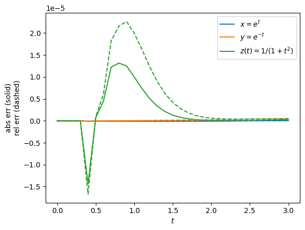
This looks pretty good, however, to check that we have implemented things correctly, we need to check that we get the predicted scaling. For this method, we know that we should have an accuracy of \(O(\d{t}^6)\) at each time-step. Thus, we expect that if we iterate \(N_t = T/\d{t}\) steps, this should degrade to \(O(\d{t}^5)\). If we don’t see this behaviour, then there is probably something wrong with our code.
T = 10.0
Nts = 2**np.arange(7, 15)
dts = T/Nts

# Get 6th derivatives
d6q_dt6 = abs(q(np.linspace(t0, T), d=6)).max(axis=1)

errs = [abs(get_errors(Nt=_Nt, T=T)[1]).max(axis=1) for _Nt in Nts]

fig, ax = plt.subplots()
ax.loglog(Nts, errs, '-+')
ax.set_prop_cycle(None)
ax.plot(Nts, 0.01*d6q_dt6[None, :]*dts[:, None]**5, '--', label='dt^5')
ax.set(xlabel='$N_t$', ylabel='maximum absolute err',
       title='dashed = $\max(y^{(6)})dt^{5}/100$')
ax.legend(labels=[r'$x=e^{t}$', r'$y=e^{-t}$', r'$z(t)=1/(1+t^2)$']);
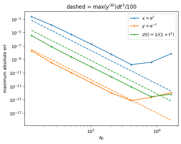
This is a pretty rigorous test: we see that our convergence is as expected - including a prefactor proportional to the sixth derivative \(y^{(6)}\). We did not compute the prefactor, but see that a prefactor of 0.01 works reasonably well. An even better test would be to compute this prefactor explicitly.