Recursion and Invariants#
Consider the famous Fibonacci numbers defined by
We code this directly in terms of recursion:
def fib0(n):
    """Return the n'th Fibonnacci number."""
    if n == 0:
        return 0
    if n == 1:
        return 1
    return fib0(n-1) + fib0(n-2)

[fib0(n) for n in range(15)]
[0, 1, 1, 2, 3, 5, 8, 13, 21, 34, 55, 89, 144, 233, 377]
If you try timing these, however, you will notice a disturbing trend:
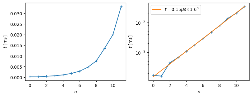
t_h = 0.13e-6 * (1.6**55) / 60**2
print(f"{t_h:.2g}h on my computer")
6.1h on my computer
If this trend continues – and it seems pretty likely – then fib(55) will take about
6 hours to compute.
Solution
How many times must fib0 recurse? Call this \(S(n)\): we have the base-cases \(S(0) =
S(1) = 1\). Then, by recursion, we must have
This means that that \(S(N)\) is just the Fibonacci series shifted by one:
Thus, the time grows in the same way as the Fibonacci series.
Can we find an explicit formula? We give two solutions here.
The Fibonacci numbers satisfy a 2-term homogeneous and linear recurrence relation:
\[\begin{gather*} F_{n} - F_{n-1} - F_{n-1} = 0. \end{gather*}\]There is an exact analogy with 2nd-order homogeneous and linear ordinary differential equations (ODEs). The following strategy generally solves these.
As with ODEs, we guess a solution of the form \(F_{n} = e^{an}\). Plugging this in, we have
\[\begin{gather*} e^{an} = e^{a(n-1)} + e^{a(n-2)} = e^{an}(e^{-a} + e^{-2a}) = e^{an}\bigl(e^{-a} + (e^{-a})^2\bigr). \end{gather*}\]Letting \(x = e^{a}\) so that \(F_{n} = e^{an} = x^n\), this becomes a quadratic equation:
\[\begin{gather*} 1 = \frac{1}{x} + \frac{1}{x^2}, \qquad x^2 - x - 1 = 0, \\ x_{\pm} = \frac{1\pm \sqrt{5}}{2}. \end{gather*}\]Since this is a two-term recurrence, there are two independent solutions, just as with a 2nd order ODE. The general solution can be expressed as
\[\begin{gather*} F_{n} = c_+ x_+^n + c_-x_-^n \end{gather*}\]where \(c+{\pm}\) ate chosen to match the initial conditions \(F_{0} = c_{+} + c_{-} = 0\), and \(F_{1} = c_+x_+ + c_-x_- = 1\). Solving this gives the complete solution:
\[\begin{gather*} F_{n} = \frac{x_+^n - x_-^n}{\sqrt{5}} = \frac{\varphi^{n} - (-\varphi)^{-n}}{\sqrt{5}}. \end{gather*}\]Note that \(x_+ = \varphi\) is the famous Golden ratio:
\[\begin{gather*} x_+ = \frac{1+\sqrt{5}}{2} = \varphi = 1.618\dots,\qquad x_- = \frac{-1}{\varphi} = 1-\varphi = -.618\dots. \end{gather*}\]Asymptotically, \(F_{n} \sim \varphi^{n}\), explaining the asymptotic time-dependence of \(1.6^{n}\) seen in the cost of
fib0. In fact:\[\begin{gather*} \DeclarePairedDelimiter{\round}⌊⌉ \DeclarePairedDelimiter{\round}\lfloor\rceil F_{n} = \round[\Big]{\varphi^{n}/\sqrt{5}} \end{gather*}\]where \(\round{x}\) means “round \(x\) to the nearest integer.
Alternatively (see [Graham et al., 1994]), one can form the generating fuction
\[\begin{alignat*}{6} f(z) &= &&F_0 + &&F_1 z + &&F_2 z^2 + && F_3 z^3 + \cdots\\ zf(z) &= && &&F_0z + &&F_1 z^2 + && F_2 z^3 + \cdots\\ z^2f(z) &=&& && &&F_0 z^2 + && F_1 z^3 + \cdots. \end{alignat*}\]Subtracting the second two from the first, and using the recurrence \(F_{n} - F_{n-1} - F_{n-2} = 0\), we have
\[\begin{gather*} (1-z-z^2)f(z) = F_0 + (F_1 - F_0) z = z, \\ f(z) = \frac{z}{1-z-z^2} = \sum_{n=0}^{\infty} F_{n}z^n. \end{gather*}\]Now we simply need to find the Maclaurin series of this function, which can be done using partial fractions and then geometric series:
\[\begin{gather*} z^2 + z - 1 = (z + \varphi)(z + 1-\varphi), \qquad \varphi = \frac{1 + \sqrt{5}}{2}\\ f(z) = \frac{z}{1-z-z^2} = \frac{-z}{(z + \varphi)(z + 1 - \varphi)} = \frac{z/\sqrt{5}}{z+1-\varphi} - \frac{z/\sqrt{5}}{z + \varphi}\\ = \frac{1}{\sqrt{5}} \left(\sum_{n=1}^{\infty} \frac{z^n}{(\varphi-1)^n} - \sum_{n=1}^{\infty} \frac{z^n}{(-\varphi)^n}\right)\\ = \sum_{n=1}^{\infty} \underbrace{\frac{1}{\sqrt{5}} \left(\frac{1}{(\varphi-1)^n} - \frac{1}{(-\varphi)^n}\right) }_{F_{n}}z^{n}. \end{gather*}\]Using the fact that \(\varphi-1 = \phi^{-1}\), we have the same result as above:
\[\begin{gather*} F_{n} = \frac{\varphi^{n} - (-\varphi)^{-n}}{\sqrt{5}}. \end{gather*}\]
1.618033988749895 -0.6180339887498948
from functools import cache

@cache
def fib0a(n):
    """Return the n'th Fibonnacci number."""
    if n == 0:
        return 0
    if n == 1:
        return 1
    return fib0a(n-1) + fib0a(n-2)

%timeit fib0a(100)
37.9 ns ± 0.146 ns per loop (mean ± std. dev. of 7 runs, 10,000,000 loops each)
From Recursion to Iteration#
One way to improve this is to accumulate the results as we go along. This turns our recursive program into an iterative program.
def fib1(n):
    F0 = 0
    F1 = 1
    while n > 0:
        F0, F1 = F1, F0 + F1
        n -= 1
    return F1
Is this correct? Perhaps we should write a test:
def test_fib(fib):
    res = list(map(fib, range(15)))
    exact = [0, 1, 1, 2, 3, 5, 8, 13, 21, 34, 55, 89, 144, 233, 377]
    if res == exact:
        return True
    else:
        print(f"{res} != {exact}")
        return False

test_fib(fib0)
True
Our test seems to work with fib0. What about fib1?
test_fib(fib1)
[1, 1, 2, 3, 5, 8, 13, 21, 34, 55, 89, 144, 233, 377, 610] != [0, 1, 1, 2, 3, 5, 8, 13, 21, 34, 55, 89, 144, 233, 377]
False
Looking at the output, we can probably guess how to fix this:
def fib1a(n):
    F0 = 0
    F1 = 1
    while n > 0:
        F0, F1 = F1, F0 + F1
        n -= 1
    return F0

test_fib(fib1a)
True
But how can we code in a way that we know our code is correct? A general approach for this strategy involves invariants.
Invariants#
Here is how we might structure our code, adding invariants so that we can ascertain the correctness of our program:
def fib2(n):
    # Invariant: F0 = F_{m}, F1 = F_{m+1}
    m = 0
    F0 = 0
    F1 = 1
    # Invariant satisfied: F0 = F_{0} = 0, F1 = F_{1} = 1

    # Check that n is a positive integer...
    assert n >= 0 and n % 1 == 0
    while m < n:
        # At the start of the loop we assume the invariant is satisfied:
        # F0 = F_{m}, F1 = F_{m+1}

        F0, F1 = F1, F0 + F1   # F0 = F_{m+1}, F1 = F_{m} + F_{m+1}
        m += 1                 # F0 = F_{m},   F1 = F_{m-1} + F_{m}

        # At the end of the loop, we check the invarient:
        # F0 = F_{m}, F1 = F_{m-1} + F_{m} = F_{m+1}
        # Invariant satisfied!

    # The loop will terminate when m == n (as long as n is an integer)
    # thus, F0 contains F_{m}
    return F0

# Now let's check to be sure
test_fib(fib2)
True