Molecular Dynamics

Hide code cell source

import mmf_setup; mmf_setup.nbinit()
import os, sys
from pathlib import Path
FIG_DIR = Path(mmf_setup.ROOT) / '../Docs/_build/figures/'
os.makedirs(FIG_DIR, exist_ok=True)
import logging; logging.getLogger("matplotlib").setLevel(logging.CRITICAL)
%matplotlib inline
import numpy as np, matplotlib.pyplot as plt
try: from myst_nb import glue
except: glue = None

from matplotlib.animation import FuncAnimation
from phys_581.contexts import FPS

This cell adds /home/docs/checkouts/readthedocs.org/user_builds/wsu-phys-581-computation/checkouts/latest/src to your path, and contains some definitions for equations and some CSS for styling the notebook. If things look a bit strange, please try the following:

  • Choose "Trust Notebook" from the "File" menu.
  • Re-execute this cell.
  • Reload the notebook.

Molecular Dynamics#

Another way to simulate material properties is with molecular dynamics (MD). This simply uses Newton’s laws to track the positions \(\vect{r}_{i}\) and velocities \(\vect{v}_{i} = \dot{\vect{r}}_{i}\) of many particles:

\[\begin{gather*} m_i\ddot{\vect{r}}_i = \vect{F}_{i}(\{\vect{r},\vect{v}\}). \end{gather*}\]

What makes MD simulations difficult is calculating the force \(\vect{F}_{i}\), which may depend on many or all of the other particles. For example, if the particles interact through a potential \(V(r)\), then we have formally

\[\begin{gather*} \vect{F}_{i}= -\sum_{j\neq i}\vect{r}_{ij}\frac{V'(\norm{\vect{r}_{ij}})} {2\norm{\vect{r}_{ij}}}, \qquad \vect{r}_{ij} = \vect{r}_{i} - \vect{r}_{j}. \end{gather*}\]

Naïvely, this requires summing over all the particles – \(O(N)\) operations – for every particle, leading to a computational complexity of \(O(N^2)\). Part of the art of MD is using clever approximations to reduce this complexity. See [Griebel et al., 2007] for details.

Lennard-Jones Potential#

A common example is to use a Lennard-Jones potential:

\[\begin{gather*} V(r) = \epsilon f\left(\frac{r}{\sigma}\right), \qquad f(q) = 4\frac{1-q^{6}}{q^{12}}, \qquad f'(q) = 24\frac{r^{6} - 2}{q^{13}} \end{gather*}\]

Hide code cell source

r = np.linspace(0, 3, 500)[1:]
f = 4/r**6*(1/r**6 - 1)
fig, ax = plt.subplots(figsize=(3,2), layout="constrained")
ax.plot(r, f)
ax.set(xlabel="$r/\sigma$", ylabel="$V(r)/\epsilon$", 
       title="Lennard-Jones Potential", ylim=(-1.1, 1));
../_images/2cac1bb42f8e269a5db4ed837c183b049e677274eb52770323c234dd31a7a5ee.png

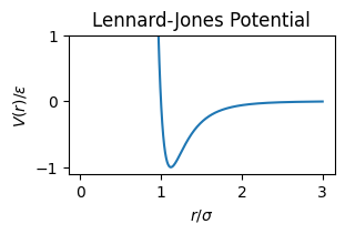
This has a minimum at \(r_\min = 2^{1/6}\sigma\) where \(V'(r_\min) = 0\), which can be used to create a stable crystalline solid, thereby allowing us to simulate the elastic properties of materials in extreme conditions (i.e., where they explode).

Time Evolution#

Care must be taken when evolving an MD simulation in time, otherwise, numerical errors will rapidly invalidate your simulation. Here we use the Velocity-Størmer-Verlet integration scheme

\[\begin{align*} \vect{r}(t+\delta t) &= \vect{r}(t) + \vect{v}(t) \delta t + \tfrac{1}{2}\vect{a}(t)\delta t^2,\\ \vect{a}(t+\delta t) &= \vect{F}\bigl(\{\vect{r}(t+\delta t)\}\bigr)/m,\\ \vect{v}(t+\delta t) &= \vect{v}(t) + \frac{\vect{a}(t) + \vect{a}(t+\delta t)}{2}\delta t. \end{align*}\]

This requires storing the previous acceleration \(\vect{a}(t)\) with each step.

Here we present a simple simulation of a projectile impacting a slab (see Fig. 3.12 of Griebel:2007). This is a simple code but runs slowly as it suffers from the \(O(N^2)\) complexity (hence the small resolution shown here).

The philosophy here is to first code the simplest thing you can to make sure we understand the essential pieces of the algorithm, and that there are no roadblocks. Once you have this, it can form a test-bed for optimizing and exploring more complicated algorithms.

Hide code cell source

_EPS = np.finfo(float).eps

class MolecularDynamics:
    L1 = 250
    L2 = 40
    epsilon = 5
    sigma = 1
    m = 1
    N1xy = (40, 40)
    N2xy = (160, 40)
    v1 = 0 - 10j
    v2 = 0 + 0j
    r_cut_sigma = 2.5
    dt = 0.00005
    beta = 0.0
    
    sep = 0+5j  # Initial separation (units of dx)

    # For colouring
    vmax = 5
    cmap = plt.colormaps['viridis']

    def __init__(self, **kw):
        for key in kw:
            if not hasattr(self, key):
                raise ValueError(f"Unknown {key=}")
            setattr(self, key, kw[key])
        self.init()
    
    def init(self):
        self.dx = 2**(1/6) * self.sigma   # Equilibrium spacing
        self.z0_1 = (-self.N1xy[0]/2 + (self.N1xy[1]-1)*1j +  self.sep) * self.dx
        self.z0_2 = (-self.N2xy[0]/2 + 0j) * self.dx
        
    def F_r(self, r2):
        """Return F/r where F is the Lennard-Jones force for separation r.
        
        I.e., F_ij = (F/r)*r
        
        where r = r_j - r_i.
        
        Arguments
        =========
        r2 : array-like
            Square of the separation distance.
        """
        # Prevent divide-by-zero errors
        r2_ = r2 + _EPS
        # s = (sigma/r)**6
        s = np.where(r2 > 0, (self.sigma**2 / r2_)**2, 0)
        s *= s**2
        f = 24 * self.epsilon * s / r2_ * (1 - 2*s)
        return f
        
    def get_initial_state(self):
        (X1, Y1), (X2, Y2) = [
            np.meshgrid(*[np.arange(N)* self.dx + x0
                          for (N, x0) in zip(Nxy, (z0.real, z0.imag))],
                        indexing='ij')
            for Nxy, z0 in [(self.N1xy, self.z0_1), 
                            (self.N2xy, self.z0_2)]
        ]
        Z1 = X1 + 1j*Y1
        Z2 = X2 + 1j*Y2
        V1 = 0*Z1 + self.v1
        V2 = 0*Z2 + self.v2
        Z, V = [np.concatenate(list(map(np.ravel, A)))
                for A in ((Z1, Z2), (V1, V2))]
        return (0, Z, V, 0*Z)
        
    def plot(self, state, ax=None):
        if ax is None:
            fig, ax = plt.subplots(layout="constrained")
        else:
            fig = ax.figure
        
        t, z, v, a = state
        ax.scatter(z.real, z.imag, c=self.cmap(abs(v)/self.vmax))
        ax.set(title=f"{t=:.4f}", aspect=1)
        return ax
    
    def get_F(self, z):
        """Return the total force on particles at z."""
        r = z[None, :] - z[:, None]
        return (self.F_r(r2=abs(r)**2) * r).sum(axis=1)
        
    def step(self, state):
        """Return the acceleration on each particle.
        
        This uses the Velocity-Størmer-Verlet method.
        """
        dt = self.dt
        t0, z0, v0, a0 = state
        z1 = z0 + dt * v0 + dt**2/2 * a0
        a1 = self.get_F(z1) / self.m
        v1 = v0 + dt / 2 * (a0 + a1)
        return (t0 + dt, z1, v1, a1)
md = MolecularDynamics()
md = MolecularDynamics(N1xy=(4*3, 4*3), N2xy=(16*3, 4*3), sep=0.4+4j)

Hide code cell source

%%time

md = MolecularDynamics(
    v1=-5j, beta=0.0, N1xy=(4*2, 4*2), N2xy=(16*2, 4*2), sep=-10.3+2j,
    dt=0.00005*40)
s = md.get_initial_state()

fig, ax = plt.subplots(layout="constrained")
for frame in FPS(100, fig=fig, embed=True):
    for n in range(20):
        s = md.step(s)
    ax.cla()
    ax = md.plot(s, ax=ax)
    ax.set(xlim=(-12*2, 12*2), ylim=(-5, 10*2))
CPU times: user 10.9 s, sys: 4.99 s, total: 15.8 s
Wall time: 17 s