Show code cell content

Hide code cell content

import mmf_setup

mmf_setup.nbinit()
import logging

logging.getLogger("matplotlib").setLevel(logging.CRITICAL)
%matplotlib inline
import numpy as np, matplotlib.pyplot as plt

$\newcommand{\vect}[1]{\mathbf{#1}} \newcommand{\uvect}[1]{\hat{#1}} \newcommand{\abs}[1]{\lvert#1\rvert} \newcommand{\norm}[1]{\lVert#1\rVert} \newcommand{\I}{\mathrm{i}} \newcommand{\ket}[1]{\left|#1\right\rangle} \newcommand{\bra}[1]{\left\langle#1\right|} \newcommand{\braket}[1]{\langle#1\rangle} \newcommand{\Braket}[1]{\left\langle#1\right\rangle} \newcommand{\op}[1]{\mathbf{#1}} \newcommand{\mat}[1]{\mathbf{#1}} \newcommand{\d}{\mathrm{d}} \newcommand{\D}[1]{\mathcal{D}[#1]\;} \newcommand{\pdiff}[3][]{\frac{\partial^{#1} #2}{\partial {#3}^{#1}}} \newcommand{\diff}[3][]{\frac{\d^{#1} #2}{\d {#3}^{#1}}} \newcommand{\ddiff}[3][]{\frac{\delta^{#1} #2}{\delta {#3}^{#1}}} \newcommand{\floor}[1]{\left\lfloor#1\right\rfloor} \newcommand{\ceil}[1]{\left\lceil#1\right\rceil} % The following allows KaTeX to render these for significantly improved % performance on CoCalc. \newcommand{\DeclareMathOperator}[2]{\newcommand{#1}{#2}} \DeclareMathOperator{\Tr}{Tr} \DeclareMathOperator{\erf}{erf} \DeclareMathOperator{\erfi}{erfi} \DeclareMathOperator{\sech}{sech} \DeclareMathOperator{\sn}{sn} \DeclareMathOperator{\cn}{cn} \DeclareMathOperator{\dn}{dn} \DeclareMathOperator{\sgn}{sgn} \DeclareMathOperator{\order}{O} \DeclareMathOperator{\diag}{diag} % \newcommand{\mylabel}[1]{\label{#1}\tag{#1}} \newcommand{\degree}{\circ}$

This cell adds /home/docs/checkouts/readthedocs.org/user_builds/wsu-phys-581-computation/checkouts/latest/src to your path, and contains some definitions for equations and some CSS for styling the notebook. If things look a bit strange, please try the following:

• Choose "Trust Notebook" from the "File" menu.
• Re-execute this cell.
• Reload the notebook.

Ordinary Differential Equations (ODEs)

Here we consider solving ODEs of the generic form

\[\begin{gather*} \dot{\vect{y}} = \vect{f}(t, \vect{y}). \end{gather*}\]

Reduction to 1st order.

All higher-order ODEs can be reduced to a system of first-order ODEs by introducing intermediate variables. For example, consider Newton’s law:

\[\begin{gather*} m\ddot{x} = F(t, x), \qquad x(0) = x_0, \qquad \dot{x}(0) = v_0. \end{gather*}\]

We can express this as the system.

\[\begin{gather*} \vect{y} = \begin{pmatrix} x(t)\\ \dot{x}(t) \end{pmatrix}, \qquad \diff{\vect{y}}{t} = \begin{pmatrix} \dot{x} = y_1\\ F(t, x)/m = F(t, y_0)/m \end{pmatrix}, \qquad \vect{y}(t) = \begin{pmatrix} x_0\\ v_0 \end{pmatrix}. \end{gather*}\]

To complete the problem we need to specify boundary conditions. The simplest form an initial-value problem (IVP) where we specify the values of \(\vect{y}(t_0) = \vect{y}_0\) at an initial time \(t=t_0\). As long as \(\vect{f}\) is single-valued, this guarantees a unique solution up to such a point as the system becomes singular.

More complicated boundary-value problems (BVPs) arise when various conditions are specified at different times. These can be generically solved using an IVP solver through a process called shooting methods that we will discuss later.

Initial Value Problems (IVPs)

Guaranteeing results with adaptive step-size selection is tricky as this essentially unsolved scipy issue #9899 shows. See the project idea Improve solve_ivp.

To get work done, I recommend using scipy.integrate.solve_ivp(), which wraps several different IVP solvers with adaptive step-size algorithms to ensure convergence. However, you should really understand what is happening under the hood. Here we will do this with a simple problem following [Gezerlis, 2023] §8.2:

\[\begin{gather*} y'(x) = \mu y(x), \qquad y(0) = 1 \tag{8.33} \end{gather*}\]

where \(\mu\) is a real constant. This has the analytic solution

\[\begin{gather*} y(x) = e^{\mu x}. \end{gather*}\]

Do It!

Write some simple code and tests to solve for \(y(x)\) with \(x\in [0, 1]\) for various step-sizes. To make this concrete, you might consider expressing your solution in terms of a function like the following:

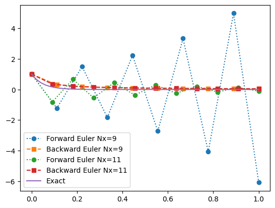
Here we reproduce Fig. 8.2 from [Gezerlis, 2023]:

mu = -20.0

def f(x, y, mu=mu):
    return mu*y
    
def solve_euler_forward(f, Nx, x0=0, x1=1, y0=1.0):
    """Solve the IVP using forward Euler."""
    xs = np.linspace(x0, x1, Nx+1)
    dx = np.diff(xs).mean()
    ys = [y0]
    for n in range(Nx):
        x, y = xs[n], ys[-1]
        dy_dx = f(x=x, y=y)
        dy = dy_dx * dx
        ys.append(y + dy)
    return xs, np.asarray(ys)


def solve_euler_backward(f, Nx, x0=0, x1=1, y0=1.0):
    """Solve the IVP using forward Euler."""
    xs = np.linspace(x0, x1, Nx+1)
    dx = np.diff(xs).mean()
    ys = [y0]
    for n in range(Nx):
        x, y = xs[n], ys[-1]
        dy_dx = f(x=x, y=y)
        ys.append(y/(1-dy_dx * dx))
    return xs, np.asarray(ys)


fig, ax = plt.subplots()
for Nx in [9, 11]:
    xs, ys = solve_euler_forward(f, Nx=Nx)
    ax.plot(xs, ys, ":o", label=f"Forward Euler {Nx=}")
    xs, ys = solve_euler_backward(f, Nx=Nx)
    ax.plot(xs, ys, "--s", label=f"Backward Euler {Nx=}")

x = np.linspace(0, 1)
ax.plot(x, np.exp(mu*x), label="Exact")
ax.legend()

<matplotlib.legend.Legend at 0x7825a2618c20>

Do It!

Explain what is happening by performing an error analysis - consider only truncation errors at this point.

What is happening can be fully understood by looking at what Euler’s method does. For this example we have

\[\begin{align*} y_{n+1} &= y_{n} + y'_{n}h, \tag{Forward}\\ y_{n+1} &= y_{n} + y'_{n+1}h. \tag{Backward} \end{align*}\]

Solving these for \(y_{n+1}\) we have

\[\begin{align*} y_{n+1} &= (1+\mu h)y_{n} = (1+\mu h)^{n-1}y_{0}, \tag{Forward}\\ y_{n+1} &= \frac{y_{n}}{1-\mu h} = \frac{y_{0}}{(1-\mu h)^{n-1}}. \tag{Backward} \end{align*}\]

Consider integrating up to \(x=1\) in \(N\) steps so that \(h = 1/N\), then \(x = nh\) and

\[\begin{align*} y(x) &= \left(1+\frac{\mu}{N}\right)^{Nx}y_{0}, \tag{Forward}\\ y(x) &= \left(1-\frac{\mu}{N}\right)^{-Nx}y_{0}. \tag{Backward} \end{align*}\]

Noting that for \(\mu < 0\), the solution \(y(x) = e^{\mu x}\) decays exponentially, we see that the forward Euler solution is unstable if \(N < -\mu\) in the sense that the solution grows rather than decays. In contrast, the backward Euler method decays for all values of \(N\) when \(\mu < 0\).

Explicit versus Implicit

Implicit methods like backward Euler are generally much more stable than explicit methods like forward Euler, but this stability comes at a cost:

\[\begin{align*} y_{n+1} &= y_{n} + f(y_{n}, x)h, \tag{Forward}\\ y_{n+1} &= y_{n} + f(y_{n+1}, x)h. \tag{Backward} \end{align*}\]

Implementing backward Euler thus requires solving a potentially non-linear equation at each step. For this reason, we generally prefer explicit methods, falling back to implicit methods only when needed.

Time-Dependent Schrödinger Equation

The time-dependent Schrödinger equation (here in 1D) is a partial differential equation:

\[\begin{gather*} \I \hbar \dot{\psi}(x, t) = \frac{-\hbar^2 \psi''(x, t)}{2m} + V(x, t)\psi(x, t). \end{gather*}\]

It can be treated as a set of coupled ODEs once we specify a procedure for computing the spatial derivatives. We will thus express it as:

\[\begin{gather*} \I \hbar \ket{\dot{\psi}(t)} = \mat{H}\ket{\psi(t)}, \qquad \ket{\psi(0)} = \ket{\psi_0} \end{gather*}\]

where \(\ket{\psi}\) is an \(N\)-component complex vector:

\[\begin{gather*} \ket{\psi} = \begin{pmatrix} \psi(x_0)\\ \psi(x_1)\\ \vdots\\ \psi(x_{N-1}) \end{pmatrix} \end{gather*}\]

consisting of the wavefunction evaluated at a set of abscissa \(\{x_n\}\), and \(\mat{H}\) is an \(N\times N\) matrix approximating the differential operator.

To start, a simple approximation can be made using finite differences

\[\begin{gather*} \psi''(x) \approx \frac{\psi(x + h) + \psi(x - h) - 2 \psi(x)}{h^2}. \end{gather*}\]

Do It!

Compute the truncation error made by this approximation: specifically, how it scales with the lattice spacing \(h\).

In this approach, we choose our abscissa to have equal “lattice” spacing \(h = x_{n+1} - x_{n}\).

For an explicit discussion of different boundary conditions, please see my classical mechanics notes Drums: Boundary Conditions. The version given here specifies Dirichlet boundary conditions.

The matrix representing the second-derivative is

\[\begin{gather*} \mat{D}_2 = \begin{pmatrix} -2 & 1 \\ 1 & -2 & 1 \\ & 1 & -2 & 1 \\ & & \ddots & \ddots & \ddots\\ & & & 1 & -2 & 1\\ & & & & 1 & -2 \end{pmatrix}. \end{gather*}\]

We can thus implement the time-dependent Schrödinger equation as a complex vector-valued ODE:

\[\begin{gather*} \ket{\dot{\psi}(t)} = \frac{1}{\I\hbar}\left( \frac{-\hbar^2}{2m}\frac{\mat{D}_2}{h^2} + \mat{\diag}V(x) \right)\ket{\psi} \end{gather*}\]

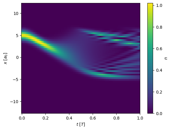
Harmonic Oscillator

Here we consider as a test case, a shifted ground state of the quantum harmonic oscillator. This state should return with the trap oscillation period, providing a test case for our code.

from scipy.integrate import solve_ivp

N = 64
L = 10.0
hbar = m = T = 1.0      # These set our units
w = 2*np.pi / T         # Angular frequency
a0 = np.sqrt(hbar/m/w)  # Oscillator length
x0 = 2.0                # Shift of initial state

t_unit = T
x_unit = a0

dx = L/N
n = np.arange(N)
x = n * dx - L/2
ones = np.ones(N)
D2 = (np.diag(ones[1:], k=1) + np.diag(ones[1:], k=-1) - 2 * np.diag(ones)) / dx**2
D2[0,0] = -1/dx**2
K = -hbar**2/2/m * D2
V = np.diag(m/2 * (w*x)**2)
H = K + V

def compute_dy_dt(t, psi):
    Hpsi = H @ psi
    return Hpsi / (1j*hbar)

# Note: It is crucial here that we make psi0 complex!
psi0 = np.exp(-((x-x0)/a0)**2/2) + 0j

res = solve_ivp(compute_dy_dt, t_span=(0, T), y0=psi0)
ts = res.t
fig, ax = plt.subplots()
psis = res.y.T
n = abs(psis)**2
mesh = ax.pcolormesh(ts / t_unit, x / x_unit, n.T)
ax.set(xlabel="$t$ [$T$]", ylabel="$x$ [$a_0$]")
plt.colorbar(mesh, label="$n$");

Aside: What is happening?

When we first solved this problem, we used \(N=64\) points and obtained the following results which look very interesting. While this is an issue of insufficient resolution, there is actually interesting physics hiding here that we now describe. To see this, note that momentum eigenstates are eigenstates of finite-difference operator:

\[\begin{gather*} \frac{\mat{D}_2}{h^2} e^{\I k x} = \frac{e^{\I k (x+h)} + e^{\I k (x-h)} - 2e^{\I k x}}{h^2} = \frac{e^{\I k h} + e^{-\I k h} - 2}{h^2}e^{\I k x}\\ = \frac{2}{h^2}\Bigl(\cos(kh) - 1\Bigr)e^{\I k x}. \end{gather*}\]

Thus, we can regard the finite-difference approximation as exactly implementing a modified Hamiltonian (modified dispersion) of the form

\[\begin{gather*} \mat{H} = K(\op{p}) + V(\op{x}), \\ K(p) = \frac{\hbar^2}{m h^2}\Bigl(1-\cos\bigl(\frac{p}{\hbar}h\bigr)\Bigr) = \frac{p^2}{2m} - \frac{p^4h^2}{24 m \hbar^2} + \cdots. \end{gather*}\]

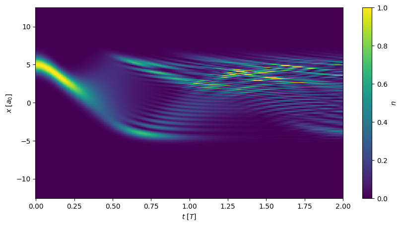
Here is a high-resolution simulation of this Hamiltonian with modified dispersion, demonstrating that the observed behaviour is indeed a result of the dispersion, and not a complete numerical artifice.

N = 256
L = 10.0
hbar = m = T = 1.0      # These set our units
w = 2*np.pi / T         # Angular frequency
a0 = np.sqrt(hbar/m/w)  # Oscillator length
x0 = 2.0                # Shift of initial state

t_unit = T
x_unit = a0

dx = L/N
n = np.arange(N)
x = n * dx - L/2
ones = np.ones(N)

h = L/64  # Value of h from previous attempt

k = 2*np.pi * np.fft.fftfreq(N, dx)
K = hbar**2 / m / h**2 * (1- np.cos(k*h))
V = m/2 * (w*x)**2

def compute_dy_dt(t, psi):
    Hpsi = np.fft.ifft(K * np.fft.fft(psi)) + V*psi
    return Hpsi / (1j*hbar)

# Note: It is crucial here that we make psi0 complex!
psi0 = np.exp(-((x-x0)/a0)**2/2) + 0j

res = solve_ivp(compute_dy_dt, t_span=(0, 2*T), y0=psi0)
ts = res.t
fig, ax = plt.subplots(figsize=(10,5))
psis = res.y.T
n = abs(psis)**2
mesh = ax.pcolormesh(ts / t_unit, x / x_unit, n.T, vmax=1)
ax.set(xlabel="$t$ [$T$]", ylabel="$x$ [$a_0$]")
plt.colorbar(mesh, label="$n$");