import mmf_setup;mmf_setup.nbinit()
import logging;logging.getLogger('matplotlib').setLevel(logging.CRITICAL)
%pylab inline --no-import-all
This cell adds /home/docs/checkouts/readthedocs.org/user_builds/wsu-phys-581-computation/checkouts/latest/src to your path, and contains some definitions for equations and some CSS for styling the notebook. If things look a bit strange, please try the following:
- Choose "Trust Notebook" from the "File" menu.
- Re-execute this cell.
- Reload the notebook.
%pylab is deprecated, use %matplotlib inline and import the required libraries.
Populating the interactive namespace from numpy and matplotlib
Assignment 1: Recursion and Invariants#
Fibonacci Numbers#
At the end of Recursion and Invariants, we showed how to use invariants to prove that a simple iterative approach for finding the n’th Fibonacci number works. Do the same with the following more sophisticated algorithm.
First note that we can write the Fibonacci recurrence in terms of a matrix equation
The idea is to use this to express the final answer in as a product of some matrix power \(\mat{M}^{p}\) times the initial conditions: (You must determine exactly what power \(p\) you need to compute \(F_{n}\).)
The strategy is to compute \(\mat{M}^{p}\) efficiently in order \(\log_2(p)\) operations. This is most easily done when \(p = 2^{q}\) is a power of 2: The idea is based on the fact that we can construct \(\mat{M}^{2^{q}}\) by repeatedly squaring the result:
To make this work for general \(p\), you will need to keep track of more information. (Hint, consider the binary representation of \(p\).)
import numpy as np
M = np.array([[1, 1],
              [1, 0]])
M2 = M @ M
M4 = M2 @ M2
print(M2)
print(M4)
[[2 1]
 [1 1]]
[[5 3]
 [3 2]]
Assignment: Efficient Fibonacci Numbers
Write a simple program to compute \(F_{n}\) based on this algorithm, and prove that it is
correct using invariants. For matrix multiplication, you can use numpy.array()
and the matrix multiplication operator.matmul() which you use as A @ B. (See
code in the margin.)
If you want to use this code in the 1ms challenge, then you need to implement your own version of matrix multiplication.
Solution
First we solve the problem of raising \(\mat{M}^{p}\). The key is to consider the binary representation of \(p\). For example, suppose \(p = 10110 = 2^4 + 2^2 + 2^1 = 22\): we can express
The strategy is to iterate through the powers of \(2^{q}\) and then accumulate those that are needed.
Using a custom implementation of matrix multiplication, I can compute up to \(F_{16383}\) on CoCalc, depending on the server load.
Evaluating Functions#
Lambert W function#
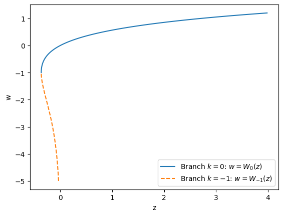
Write a function phys_581.assignment_1.lambertw() that computes \(w = W_k(x)\), the
Lambert W function, for the two
branches \(k=0\) and \(k=-1\).
This function satisfies:
and \(k\) determines which branch you should compute as shown below:
w0 = np.linspace(-1, 1.2, 100)
w1 = np.linspace(-5, -1, 100)
fig, ax = plt.subplots()
for w, k, ls in [(w0, 0, '-'), (w1, -1, '--')]:
    z = w*np.exp(w)
    ax.plot(z, w, linestyle=ls,
            label=f"Branch $k={k}$: $w=W_{{{k}}}(z)$")
ax.legend()
ax.set(xlabel='z', ylabel='w');
Riemann zeta function#
Write a function phys_581.assignment_1.zeta() that computes the Riemann zeta
function
Make sure your function returns a result with relative accuracy within a few orders of magnitude of machine precision for all values of \(s > 1\) where the result does not overflow.
Differentiation#
Write a function phys_581.assignment_1.derivative() that numerically computes the
derivatives of a function \(f(x)\) at a point \(x\):
from phys_581.assignment_1 import derivative

x = 1.0
for d, exact in [
    (0, np.sin(x)),
    (1, np.cos(x)),
    (2, -np.sin(x)),
    (3, -np.cos(x)),
    (4, np.sin(x))
]:
    res = derivative(np.sin, x=x, d=d)
    rel_err = abs(res-exact)/abs(exact)
    print(f"d={d}: numeric={res:.8g}, exact={exact:.8g}, rel_err={rel_err:.4g}")
d=0: numeric=0.84147098, exact=0.84147098, rel_err=0
d=1: numeric=0.54030231, exact=0.54030231, rel_err=1.783e-11
d=2: numeric=-0.84147085, exact=-0.84147098, rel_err=1.578e-07
d=3: numeric=-0.58243278, exact=-0.54030231, rel_err=0.07798
d=4: numeric=-30177.269, exact=0.84147098, rel_err=3.586e+04
The default code carefully chooses an optimal value of \(h\) as discussed below, then uses a recursive approach to compute higher derivatives. Can you improve the accuracy of this?
Bonus: Why does the following trick work to machine precision?
def derivative1(f, x):
    """Compute the first 1 derivative extremely accurately for *some* functions."""
    h = 1e-64j
    return ((f(x+h) - f(x))/h).real

print(f"f=sin(x): err = {abs(derivative1(np.sin, x) - np.cos(x))}")
print(f"f=exp(x): err = {abs(derivative1(np.exp, x) - np.exp(x))}")
f = lambda x: np.exp(-x**2)
df = lambda x: -2*x*np.exp(-x**2)
print(f"f=exp(-x**2): err = {abs(derivative1(f, x) - df(x))}")
f=sin(x): err = 0.0
f=exp(x): err = 0.0
f=exp(-x**2): err = 0.0
More Details#
Roundoff vs Truncation Error#
Consider computing the derivative of a function using finite-difference techniques:
We can estimate the error computing this by using the Taylor series for the function:
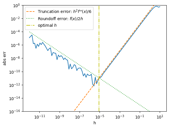
This forward-difference approximation thus has a truncation-error that scales as \(hf''(x)/2\). We can do a bit better if we take the centered-difference approximation:
However, this is not the only source of error. If all goes well, the values \(f(x\pm h)\) will be computed with a relative error of machine precision \(\epsilon\), which means they will have have an absolute error of \(\approx \epsilon f(x)\). Dividing this error by \(2h\), however, means that the whole expression will have an absolute error of about \(\epsilon f(x)/2h\) because of roundoff error. Notice that this gets significantly worse as \(h\) gets small.
With this formula, the best we can do is to choose
The following plot shows that these estimates are accurate.
eps = np.finfo(float).eps
h = 10 ** np.linspace(-12, 1, 100)
x = 1.0
f = np.sin
df = np.cos
d3f = lambda x: -np.sin(x)
Df_x = (f(x + h) - f(x - h)) / 2 / h  # Centered difference approx
err = abs(Df_x - df(x))
truncation_err = abs(h ** 2 * d3f(x) / 6)
roundoff_err = abs(eps * f(x) / 2 / h)
h_opt = (3*eps*abs(f(x)/d3f(x)))**(1/3)
fig, ax = plt.subplots()
ax.loglog(h, err)
ax.plot(h, truncation_err, "--", label="Truncation error: $h^2 f'''(x)/6$")
ax.plot(h, roundoff_err, ":", label="Roundoff error: $f(x)/2h$")
ax.axvline(h_opt, c='y', ls='-.', label='optimal $h$')
ax.set(xlabel="h", ylabel="abs err", ylim=(1e-16, 1))
ax.legend()
<matplotlib.legend.Legend at 0x7eaf0e0a5950>
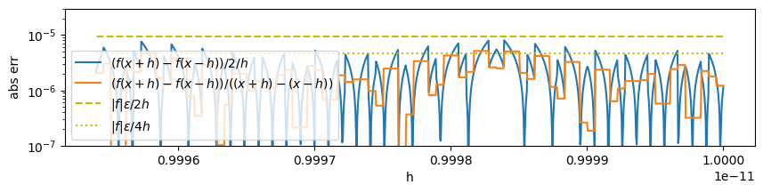
Notice that the truncation error is smooth, but the roundoff error appears random. As Alex discusses [Gezerlis, 2020] (see Fig. 2.3), roundoff errors are not random. We can see this by zooming in:
eps = np.finfo(float).eps
h = 10 ** np.linspace(-11, -11.0002, 1000)
Df_x = (f(x + h) - f(x - h)) / 2 / h  # Centered difference approx
err = abs(Df_x - df(x))

# Slightly better approach.  Compute denominator to include some roundoff error.
h2 = (x+h) - (x-h)
Df_x2 = (f(x + h) - f(x - h)) / h2  # Centered difference approx
err2 = abs(Df_x2 - df(x))

fig, ax = plt.subplots(figsize=(10,2))
ax.semilogy(h, err, label="$(f(x+h) - f(x-h))/2/h$")
ax.semilogy(h, err2, label="$(f(x+h) - f(x-h))/((x+h) - (x-h))$")
ax.plot(h,  abs(f(x)*eps) / 2 / h, "--y", label="$|f|\epsilon/2h$")
ax.plot(h, abs(f(x)*eps / 2) / 2 / h, ":y", label="$|f|\epsilon/4h$")
ax.set(xlabel="h", ylabel="abs err", ylim=(1e-7, 3e-5))
ax.legend();
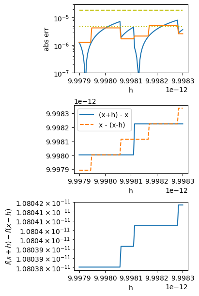
If you want to understand this in detail, consider the structure near \(h=0.9998\times 10^{-11} \approx 2^{-36}\) shown in the margin. This shows that \(h\) is small enough that \(x+h\) and \(x-h\) step through only a few different values due at machine precision.
Assignment: Floating Point Representation
Write a function that prints a summary of the floating point representation of a given number. See the code below for some hints (and useful python tools).
import struct   # Tools for unpacking bits of data
import numpy as np

pi = np.pi

print(np.finfo(pi))  # Floating point info about the variable.
Machine parameters for float64
---------------------------------------------------------------
precision = 15   resolution = 1e-15
machep = -52   eps =        2.220446049250313e-16
negep =  -53   epsneg =     1.1102230246251565e-16
minexp = -1022   tiny =       2.2250738585072014e-308
maxexp = 1024   max =        1.7976931348623157e+308
nexp =   11   min =        -max
smallest_normal = 2.2250738585072014e-308   smallest_subnormal = 5e-324
---------------------------------------------------------------
Here are some ways of manipulating data and types.
# Convert the type of a numpy scalar so we can get the dtype:
pi_ = np.array(pi)
pi_.dtype
dtype('float64')
You can query the numpy.dtype object for information. Once you have an
array, you can view() it as an integer:
pi_.view(np.uint64)
array(4614256656552045848, dtype=uint64)
This can then be converted to a binary number with the bin() function. The
result is a string that we might need to zero-pad to get the full 64-bit representation:
bin_str = bin(pi_.view(np.uint64))
print(bin_str)
print(f"{bin_str[2:].zfill(64)}")  # Strip of `0b` prefix, then zero-pad for 64 bits
0b100000000001001001000011111101101010100010001000010110100011000
0100000000001001001000011111101101010100010001000010110100011000
Which portion of these bits are the mantissa? Sign? Exponent? etc. Hint:
bin(int(pi * 2**53))
'0b1100100100001111110110101010001000100001011010001100000'
References#
numpy/numpy#10288: Meaning of
np.float128… it is not IEEE 128.