Assignment 4: Modeling Data#
In this assignment you will test your model against sample “experimental” in order to try to make a “discovery” with properly quantified errors and confidence values. In these notes, we will perform a sample analysis with a periodic signal, but you should use your chosen model for your analysis.
Project Preparation Details
Create a project on GitLab in the Physics 581-2025 group.
Clone to local computer.
Initialize:
pixi init --format pyproject.toml
pixi init --format pixi
pixi add matplotlib scipy uncertainties emcee notebook jupytext tqdm \
         pytest pytest-cov \
         mystmd
Commit
hg com -m "Initial commit of project"
Add some source code and tests etc. I am still playing with [pixi][], so here is what my init files look like:
# pyproject.toml
[project]
authors = [{name = "Michael McNeil Forbes", email = "michael.forbes+numpy@gmail.com"}]
dependencies = []
name = "data_fitting"
requires-python = ">= 3.11"
version = "0.1.0"

[build-system]
build-backend = "hatchling.build"
requires = ["hatchling"]
# pixi.toml
[workspace]
authors = ["Michael McNeil Forbes <michael.forbes+numpy@gmail.com>"]
channels = ["conda-forge"]
name = "data_fitting"
platforms = ["win-64", "linux-64", "osx-arm64", "osx-64"]
version = "0.1.0"

[tasks]

[dependencies]
matplotlib = ">=3.10.7,<4"
scipy = ">=1.16.2,<2"
uncertainties = ">=3.2.3,<4"
emcee = ">=3.1.6,<4"
notebook = ">=7.4.7,<8"
jupytext = ">=1.18.1,<2"
tqdm = ">=4.67.1,<5"
pytest = ">=8.4.2,<9"
pytest-cov = ">=7.0.0,<8"
mystmd = ">=1.6.3,<2"

[pypi-dependencies]
# Make sure this name matches the name in `pyproject.toml`.
data_fitting = { path = ".", editable = true }
$ tree
.
|-- pixi.lock
|-- pixi.toml
|-- pixi.toml_
|-- pyproject.toml
`-- src
    `-- data_fitting
        |-- __init__.py
        `-- signal1.py
GitLab Pages: We can host our documentation on GitLab using their GitLab Pages feature:
To do this we do the following:
Make sure that you can build and view static html documentation:
pixi run myst -d build --html
open _build/html/index.html
Create the following
.gitlab-ci.ymlfile. This will run the previous command using the GitLab Continuous Integration (CI) feature whenever your commit message containsDOC.# .gitlab-ci.yml image: ubuntu:24.04 build-docs: script: # - export # Useful for debugging variables. - apt-get update && apt-get install -y curl unzip # build-essential curl unzip # texlive-full - bash <(curl -fsSL https://pixi.sh/install.sh) - export PATH="$HOME/.pixi/bin:$PATH" - export BASE_URL="${CI_PAGES_URL}" - pixi install - pixi run myst -v - pixi run myst -d build --html - mv _build/html public pages: true # specifies that this is a Pages job artifacts: paths: - public rules: # Only run the CI if the commit message has "DOC" in it. - if: $CI_COMMIT_MESSAGE =~ "/DOC/"
Make these pages visible on GitLab under your project settings:
Settings -> General -> Visibility, project features, permissions: ChangesPagestoEveryone With Acecss.Deploy -> Pages -> Domains & settings: UncheckUse unique domain.
Push your documentation with
DOCin the commit message.
This should trigger a pipeline which will build and deploy the documentation. You should then be able to view it at, e.g.:
https://wsu-courses.gitlab.io/physics-581-2025/data-fitting/
See the exact URL on your GitLab project under Deploy -> Pages.
Scenario#
Imagine that your colleagues have performed an expensive experiment and obtained a small number \(N_d\) of sets of data consisting of tabulated data \(D_{d} = \{(x_n, y_n)\}\) which you believe are generated from your model
where \(\vect{a}\) are unknown parameters, and \(e_{n}\) are the experimental errors.
Your task is to learn as much as possible about the parameters \(\vect{a}\) from the data, and to express this succinctly and accurately. In particular, you should provide:
An estimate of the “best fit” values of the parameters \(\vect{a}\).
An estimate of the errors/uncertainties in these parameters.
A statistical measure of the goodness-of-fit.
(See the discussion at the end of section 15.0.0 of [Press et al., 2007].)
Here we will use the least squares approach, attempting to find parameters \(\vect{a}\) that minimize
The minimum \(\bar{\vect{a}}\) here will provides the first objective, the parameter estimates. Near this, \(\chi^2(\vect{a})\) will be quadratic:
The matrix \(\mat{C}\) is called the covariance matrix. This will form the basis for our characterization of the errors or uncertainties in the parameters. The uncertainties in the parameters will be characterized by ellipsoids of constant \(\chi^2(\vect{a})\).
Finally, we shall see that under appropriate conditions – namely, that the \(e_n\) be normally distributed and that the model \(f(x, \vect{a})\) is approximately linear over the region of parameter uncertainties – then we can characterize the distribution of \(\chi^2(\vect{a})\) to determine the confidence region. Specifically, in this case, the reduced chi-square statistic \(\chi^2_r \approx 1\) should be close to 1 if the model is good and the errors have been appropriately characterized:
Important
If the errors \(e_n\) are normally distributed, and the model is linear, then you can use the results in section 15.6.5 of [Press et al., 2007] to determine which contours of constant \(\chi^2(\vect{a})\) correspond to which confidence regions.
If the errors are not normally distributed, then you should not rely on \(\chi^2_r(\vect{a})\) to characterize your goodness-of-fit, or your confidence regions. Instead you must perform a Monte Carlo simulation to see how \(\chi^2(\vect{a})\) is distributed, then from this determine the contours of \(\chi^2(\vect{a})\) which correspond to which contour region.
If you model is not sufficiently linear, then you likely need to consider more advanced techniques such as MCMC to characterize your uncertainties, which will likely be more complicated regions than ellipsoids in parameter space.
Model: Periodic Signals#
Here we will work with the following model, looking for periodic signals in data:
Our primary focus here will be to find the frequency \(\omega\) or period \(T=2\pi / \omega\) (and possibly the phase \(\phi\)). The other parameters \(c\), \(A\), (and \(\phi\)) are called nuisance parameters: we need to include them in our analysis, but we don’t really care about their values.
Obtaining Fits#
Before looking at real data, it is a good idea to generate some sample data with known errors, and see what this means. Here we start without thinking too much, applying the standard approach of least squares fitting.
from collections import namedtuple
from uncertainties import correlated_values, unumpy as unp

Nt = 100
t_max = 10.0

# Exact parameter values
Params = namedtuple("Params", ["w", "c", "A", "phi"])
w, c, A, phi = a_exact = Params(w=2 * np.pi / 5, c=1.2, A=3.4, phi=5.6)


def f(t, w, c, A, phi):
    """Model function."""
    return c + A * np.cos(w * t + phi)


def f_wrong(t, w, c, A, phi):
    """Wrong model function."""
    return c + A * np.cos(w * t + phi) ** 3


# Exact data and experimental errors
t = np.linspace(0, t_max, Nt)
y = f(t, *a_exact)
sigmas = 0.5 * np.ones(Nt)
wrong_sigmas = sigmas / 2.0

rng = np.random.default_rng(seed=2)
ydata = rng.normal(loc=y, scale=sigmas)
<matplotlib.legend.Legend at 0x756301017d90>
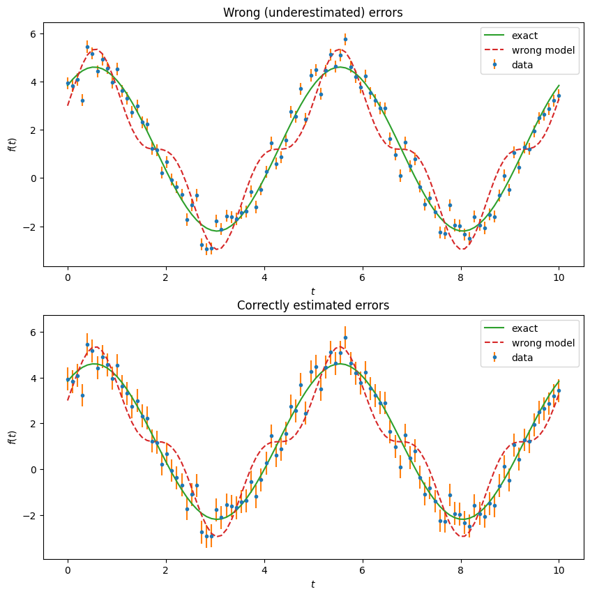
Important
Look closely at the errors in the bottom figure and how they do not all overlap the exact model. These are \(1\sigma\) error bars, meaning that about 68% of the time, the data should lie within this distance from the model, but that 32% of the data should lie further away. As we have carefully generated the deviations here, this gives a visual idea of what a model and consistent data (with errors) should look like. Can you “see” that the wrong model is inconsistent with the data and errors?
We perform three fits to demonstrate the different functions available in SciPy. Note:
we use the wrong_sigmas here which underestimate the errors by a factor of 2. This
will result in an excessively large \(\chi^2_r \gg 1\), and demonstrate the meaning of the
absolute_sigma=False flag provided by curve_fit that effectively scales the errors
so that \(\chi^2_r = 1\) before providing the covariance matrix \(\mat{C}\).
Defined function show() for displaying parameter estimates
curve_fit#
scipy.optimize.curve_fit is a good choice for fitting data to a curve. It provides
the covariance matrix with the option of automatically scaling of the errors to get a
reduced \(\chi^2_r = 1\) if you don’t know the absolute magnitude of the errors.
This routine takes your model function f(x, p1, p2, ...) and your data as an input.
If you do not provide a guess, it will try a guess of ones.
from scipy.optimize import curve_fit

nu = len(t) - len(a_exact)
a, C = curve_fit(
    f=f, xdata=t, ydata=ydata, p0=a_exact, sigma=wrong_sigmas, absolute_sigma=True
)
a_ = Params(*correlated_values(a, covariance_mat=C))
chi2_r = (((f(t, *a) - ydata) / wrong_sigmas) ** 2).sum() / nu

print("Fit with wrong errors (too small)")
show(a_)
print(f"chi^2_r = {chi2_r:.2g}")

print("\nAfter scaling C*chi^2_r - same as absolute_sigma=False")
a_ = Params(*correlated_values(a, covariance_mat=C * chi2_r))
show(a_)

a, C = curve_fit(
    f=f, xdata=t, ydata=ydata, p0=a_exact, sigma=wrong_sigmas, absolute_sigma=False
)
a_ = Params(*correlated_values(a, covariance_mat=C))
show(a_)

print("\nFit with wrong model.")
a_wrong, C_wrong = curve_fit(
    f=f, xdata=t, ydata=ydata, p0=a_exact, sigma=sigmas, absolute_sigma=True
)
chi2_r_wrong = (((f_wrong(t, *a_wrong) - ydata) / sigmas) ** 2).sum() / nu
a_wrong_ = Params(*correlated_values(a_wrong, covariance_mat=C_wrong))
show(a_wrong_)
print(f"chi^2_r = {chi2_r_wrong:.2g}")

print("\nFit with correct errors and model")
a, C = curve_fit(
    f=f, xdata=t, ydata=ydata, p0=a_exact, sigma=sigmas, absolute_sigma=True
)
a_ = Params(*correlated_values(a, covariance_mat=C))
chi2_r_correct = (((f(t, *a) - ydata) / sigmas) ** 2).sum() / nu
show(a_)
print(f"chi^2_r = {chi2_r_correct:.2g}")
Fit with wrong errors (too small)
Params(w=1.2542(38),c=1.201(26),A=3.415(35),phi=5.613(23))
chi^2_r = 3.8

After scaling C*chi^2_r - same as absolute_sigma=False
Params(w=1.2542(73),c=1.201(51),A=3.415(69),phi=5.613(44))
Params(w=1.2542(73),c=1.201(51),A=3.415(69),phi=5.613(44))

Fit with wrong model.
Params(w=1.2542(76),c=1.201(52),A=3.415(71),phi=5.613(46))
chi^2_r = 3.6

Fit with correct errors and model
Params(w=1.2542(76),c=1.201(52),A=3.415(71),phi=5.613(46))
chi^2_r = 0.94
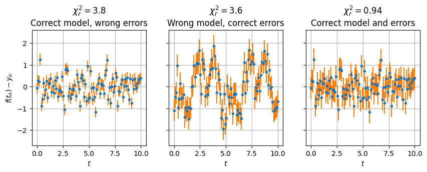
The last result is what you should be aiming for. Here we have used a correct estimate of the errors, and found that \(\chi^2_r = \) . This gives us the third component of model fitting – a statistical measure of the goodness-of-fit that is valid if the errors are small enough that a linear approximation to the model is valid. We should check this (we will below), but if it is valid, then we can trust the other parts – the parameter estimates and their correlated uncertainties.
Important
In the other cases, the large value \(\chi^2_r = \) indicates that something is wrong, and we must be very careful interpreting the results. If (and only if) we are confident in the errors (as we should be) then we can use this to reject the model as an exceedingly unlikely explanation of the data, even though the model “looks” good (“chi-by-eye”).
However, if, after plotting the residuals, it looks like there are no systematic
deviations and the residuals look flat as they do on the left, then one might reasonably
suspect that the errors have been underestimated. Go back to the experimentalists and
see if something is wrong. In the meantime, you might consider using the
absolute_sigma=False option to get estimates of the parameter uncertainties while
you wait, but don’t publish until you understand why your \(\chi^2_r\) is so large.
If the model is incorrect, then one typically sees some sort of systematic deviations like the periodic peak structure in the middle plot. In this case, the parameter estimates and values do not really have any meaning, and should be discarded until a better model is found.
least_squares#
scipy.optimize.least_squares is a bit more general. This function needs to be
provided with the list of weighted residuals:
and will the minimize the cost function
You could customize this, for example, to allow fitting of complex-valued data. You must provide an initial guess for the parameter values here.
To construct the covariance matrix, you can use the returned Jacobian:
To reproduce the results of curve_fit with absolute_sigma=False, you can normalize
this by \(\chi^2_r\):
from scipy.optimize import least_squares


def get_errors(a):
    return (f(t, *a) - ydata) / wrong_sigmas


res = least_squares(fun=get_errors, x0=a_exact)

a = res.x
J = res.jac
C = np.linalg.inv(J.T @ J)
a_ = Params(*correlated_values(a, covariance_mat=C))
nu = len(t) - len(a)
chi2_r = (get_errors(a) ** 2).sum() / nu

print("Fit with wrong errors (too small)")
show(a_)
print(f"chi^2_r = {chi2_r:.2g}")

a_ = Params(*correlated_values(a, covariance_mat=C * chi2_r))
print()
print("After scaling errors to get chi^2_r=1")
show(a_)
Fit with wrong errors (too small)
Params(w=1.2542(38),c=1.201(26),A=3.415(35),phi=5.613(23))
chi^2_r = 3.8

After scaling errors to get chi^2_r=1
Params(w=1.2542(73),c=1.201(51),A=3.415(69),phi=5.613(44))
minimize#
scipy.optimize.minimize is a generic minimizer. This provides you with the most
flexibility, but you must provide the objective function and carefully scale the results
to get the covariance matrix. As can be deduced from least_square, you will get the
correct covariance matrix \(\mat{C} = \mat{H}^{-1}\) where \(\mat{H}\) is the hessian
(second-derivative matrix) of the objective. However, if you do this, you will likely
have issues with tolerances because minimize expects the objective function to have an
optimal value close to 1.
Instead, we should use the reduced \(\chi^2_r\) as an objective, which will require scaling the hessian to get the parameter covariance matrix:
from scipy.optimize import minimize


def get_chi2_r(a):
    errors = (f(t, *a) - ydata) / wrong_sigmas
    nu = len(t) - len(a)
    return (abs(errors) ** 2).sum() / nu


res = minimize(fun=get_chi2_r, x0=a_exact, method="BFGS", tol=1e-6)

print(res.message)
assert res.success
a = res.x
nu = len(t) - len(a)
C = res.hess_inv / (nu / 2)
a_ = Params(*correlated_values(a, covariance_mat=C))
chi2_r = get_chi2_r(a)

print("Fit with wrong errors (too small)")
show(a_)
print(f"chi^2_r = {chi2_r:.2g}")

print()
a_ = Params(*correlated_values(a, covariance_mat=C * chi2_r))
print("After scaling errors to get chi^2_r=1")
show(a_)
Desired error not necessarily achieved due to precision loss.
---------------------------------------------------------------------------
AssertionError                            Traceback (most recent call last)
Cell In[9], line 13
     10 res = minimize(fun=get_chi2_r, x0=a_exact, method="BFGS", tol=1e-6)
     12 print(res.message)
---> 13 assert res.success
     14 a = res.x
     15 nu = len(t) - len(a)

AssertionError:
Changing Variables#
Once we have established the best fit parameters \(\vect{a}\) and covariance matrix \(\mat{C} = \mat{C}^T\) we have the following model about the minimum \(\bar{\vect{a}}\):
Once we have these results, we might want to consider other parameter combinations \(\vect{b} = \vect{g}(\vect{a})\). We can immediately transform these results if the \(\vect{g}(\vect{a})\) is sufficiently linear about \(\bar{\vect{a}}\):
This type of transformation can be done automatically by the uncertainties package,
which propagates the correlated errors through any arithmetic operations and non-linear
functions in the uncertainties.umath or uncertainties.unumpy modules. For example,
in our model, we might want to consider the time at which the periodic signal is a
maximum, rather than the phase:
If \(\phi\) and \(\omega\) had independent gaussian errors, then we could use standard error analysis techniques to deduce that the relative error in \(t_0\) would be the sum of the squares of the relative errors in \(\phi\) and \(\omega\):
from uncertainties import ufloat, covariance_matrix, correlated_values

a_ = Params(*correlated_values(a, covariance_mat=C))

w = a_.w
# Make phi lie between -2*np.pi and 0 so t0 is positive
phi = a_.phi % (2 * np.pi) - 2 * np.pi
t0 = -phi / w
print(f"Correlated   w={w:.3uS}, phi={phi:.3uS}, t0={t0:.3uS}")

# Now compute result as if errors were uncorrelated
w_ = ufloat(w.n, w.s)
phi_ = ufloat(phi.n, phi.s)
t0_ = -phi_ / w_
print(f"Uncorrelated w={w_:.3uS}, phi={phi_:.3uS}, t0={t0_:.3uS}")
dt0 = t0.n * np.sqrt((w.s / w.n) ** 2 + (phi.s / phi.n) ** 2)
print(f"Error from uncorrelated error formula dt0 = {dt0:.3g}")
Correlated   w=1.25424(378), phi=-0.6702(228), t0=0.5343(168)
Uncorrelated w=1.25424(378), phi=-0.6702(228), t0=0.5343(183)
Error from uncorrelated error formula dt0 = 0.0183
/tmp/ipykernel_4099/1820333103.py:7: FutureWarning: AffineScalarFunc.__mod__() is deprecated. It will be removed in a future release.
  phi = a_.phi % (2 * np.pi) - 2 * np.pi
We see here that the computed error in \(t_0\) from the actual parameters is comparable but slightly less than the estimate given by the uncorrelated error formula above. This is because the errors in \(\omega\) and \(\phi\) have some correlations as can be seen in the off-diagonal entries of the 2-parameter covariance matrix:
covariance_matrix([phi, w])
[[np.float64(0.000521378072136006), np.float64(-7.69544723296118e-05)],
 [np.float64(-7.69544723296118e-05), np.float64(1.4304206417483636e-05)]]
Principal Component Analysis (PCA)#
By diagonalizing the symmetric covariance matrix \(\mat{C} = \mat{C}^T\), we can perform a [principal component analysis] (PCA). We note that about the minimum \(\bar{\vect{a}}\), we have the model:
By diagonalizing the covariance matrix, we can find the “principal components” – those linear combinations of the original parameters that are most tightly constrained by the data:
In this new basis, we have the model
The columns of \(\vect{V}\) thus define an orthonormal basis (hence \(\mat{V}^T = \mat{V}^{-1}\)) for parameter space such that the linear combinations of parameters along these directions \(\lambda_i\) are independent, and normally distributed with variance \(\sigma_i^2\).
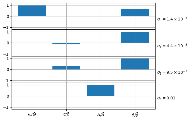
Note that the \(\lambda_i\) parameters represent linear combinations of the physical parameters \(\vect{a}\). While these are well defined, the eigenvectors themselves \(\vect{v}_i\) may not make much sense unless the original variables \(\vect{a}\) are appropriately scaled to make the components of the eigenvectors compatible. One such option is to scale each parameter by its best fit value \(\bar{\vect{a}}\), then we can write:
where the \(\vect{v}_i \bar{\vect{a}}\) and \(\delta \vect{a}/\bar{\vect{a}}\) denote element-wise multiplication and division respectively. The vectors \(\tilde{v}_i\) now provide a PCA of the relative errors, and it is often instructive to plot the components of these vectors:
from uncertainties.unumpy import nominal_values
def num2tex(x, digits=2, min_power=-2, max_power=3):
"""Return a nice LaTeX string for the number."""
power = int(np.floor(np.log10(abs(x))))
mantissa = x / 10 ** power
if min_power <= power and power <= max_power:
mantissa = mantissa * 10 ** power
format = f"{{:.{digits}g}}"
elif power == 1:
format = rf"{{:.{digits-1}f}}\times 10"
else:
format = rf"{{:.{digits-1}f}}\times 10^{{{{{{}}}}}}"
return format.format(mantissa, power)
def plot_pca(a, C, labels=None, relative=True):
"""Draw a PCA eigenvector plot.
Arguments
---------
a : Params
Parameter values
C : array
Covariance matrix
labels : [str]
Labels for the parameters (will use `a._fields` if `None`)
"""
if labels is None:
labels = p._fields
d, V = np.linalg.eigh(C)
assert np.allclose((V * d[np.newaxis, :]) @ V.T, C)
if relative:
V *= a[:, np.newaxis]
labels = [fr"${_l}/\bar{{{_l}}}$" for _l in labels]
else:
labels = list(map("${}$".format, labels))
fig, axs = plt.subplots(len(a), 1, gridspec_kw=dict(hspace=0), sharex=True)
is_ = np.arange(len(a_))
for i, ax, sigma2, v, label in zip(is_, axs, d, V.T, labels):
# Normalize so maximum component is 1
ind = np.argmax(abs(v))
_fact = v[ind]
sigma = np.sqrt(sigma2 / _fact ** 2)
ax.bar(is_, v / _fact)
ax.set(ylim=(-1.2, 1.2))
ax.yaxis.set_label_position("right")
ax.set_ylabel(fr"$\sigma_{i} = {num2tex(sigma)}$", ha="left", rotation=0)
ax.grid(True)
ax.set_xticks(is_)
ax.set_xticklabels(labels)
plot_pca(a, C, labels=[r"\omega", r"c", r"A", r"\phi"])
display(plt.gcf())
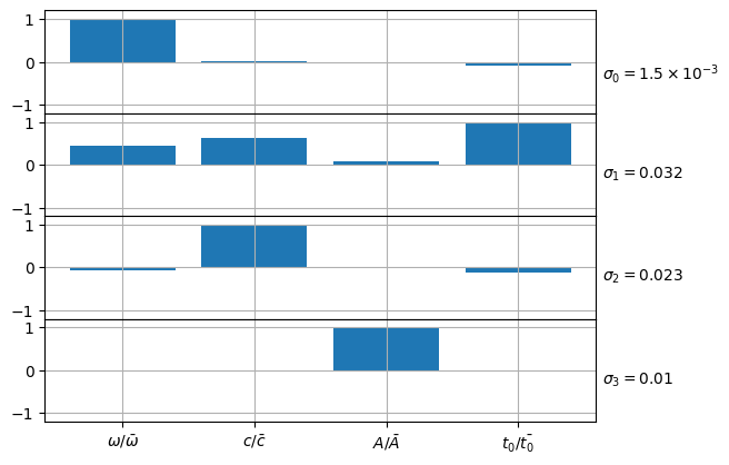
# New parameters with t0 instead of w. Note that the uncertainties package
# can construct a covariance matrix from any set of parameters.
p_new = np.concatenate([a_[:3], [t0]])
C_new = covariance_matrix(p_new)
plot_pca(nominal_values(p_new), C_new, labels=[r"\omega", r"c", r"A", r"t_0"])
display(plt.gcf())
plt.close("all")
show(a_)
show(Params(*(a_ / a)))
Params(w=1.2542(38),c=1.201(26),A=3.415(35),phi=5.613(23))
Params(w=1.0000(30),c=1.000(22),A=1.000(10),phi=1.0000(41))
show(Params(*correlated_values(a, C)))
np.sqrt(np.diag(C / a[:, None] / a[None, :]))
np.sqrt(np.diag(C))
Params(w=1.2542(38),c=1.201(26),A=3.415(35),phi=5.613(23))
array([0.00378209, 0.02621777, 0.03534004, 0.0228337 ])
Correlated Errors and the Covariance Matrix#
The covariance matrix \(\mat{C}\) describes the local dependence of \(\chi^2\) on the deviations \(\delta\vect{a} = \vect{a} - \bar{\vect{a}}\) from the best fit values:
We should check this to be sure. Note that if we vary a single parameter \(a_i\) while holding the others fixed, then we should find:
This is easy to check numerically
a, C = curve_fit(
    f=f, xdata=t, ydata=ydata, p0=a_exact, sigma=sigmas, absolute_sigma=True
)
a_ = Params(*correlated_values(a, covariance_mat=C))

def get_chi2(a, i=0, dai=0):
    a_ = np.copy(a)
    a_[i] += dai
    return (((f(t, *a_) - ydata) / sigmas)**2).sum()

Cinv = np.linalg.inv(C)

fig, ax = plt.subplots()
chi2 = get_chi2(a=a)
for i in range(len(a)):
    sigma_i = 1/np.sqrt(Cinv[i,i])
    dais = np.linspace(-sigma_i, sigma_i, 30)
    chi2s = [get_chi2(a=a, i=i, dai=dai) - chi2 for dai in dais]
    l, = ax.plot(dais, chi2s, "--", label=f"$a_i$ = {Params._fields[i]}")
    ax.plot(dais, dais**2 / sigma_i**2, ".", c=l.get_c())
ax.set(xlabel="$a_i$", ylabel=r"$\delta\chi^2$")
ax.legend();
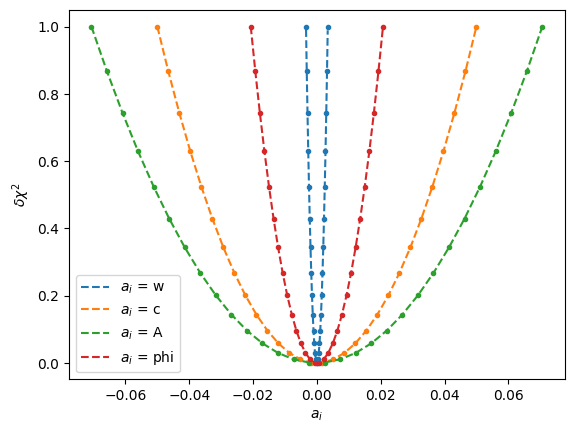
Here we see that our interpretation of the diagonals of \(\mat{C}^{-1}\) correspond with the behavior of \(\chi^2\). This supports the following interpretation of the diagonal elements of \(\mat{C}^{-1}\) and \(\mat{C}\):
The diagonal elements \(\sigma'_i = 1/\sqrt{[\mat{C}^{-1}]_{ii}}\) tell us how much we can vary the parameter \(a_i\) away from the best fit value before \(\chi^2\) changes by 1 while holding the other parameters fixed. I.e. \(a_i \in (\bar{a}_i \pm \sigma'_{i})\).
The diagonal elements \(\sigma_i = \sqrt{\mat{C}_{ii}}\) tell us how much we can vary the parameter \(a_i\) away from the best fit value before \(\chi^2\) changes by 1 while re-minimizing over the other parameters fixed.
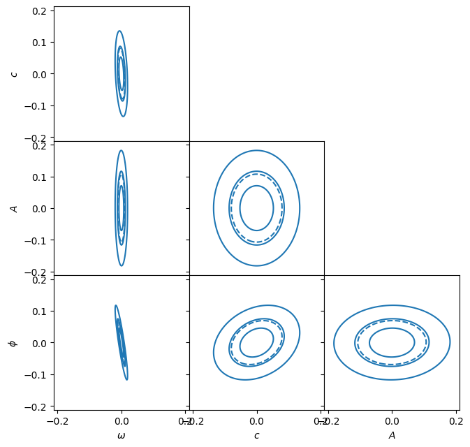
Thus, we can describe the distribution of parameters as ellipsoids of constant \(\delta\chi^2\):
To plot these in 2D, we can factor \(\mat{C} = \mat{L}\cdot\mat{L}^T\) using either a Cholesky decomposition or the same diagonalization as performed above in the PCA: \(\mat{C} = \mat{V}\cdot\mat{D}\cdot\mat{V}^T\), \(\mat{L} = \mat{V}\cdot\sqrt{\mat{D}}\). We then have:
Thus, the ellipsoids of constant \(\chi^2\) are spheres in the space \(\vect{x}\). We can now plot these pairwise in a “corner plot”:
a, C = curve_fit(
    f=f, xdata=t, ydata=ydata, p0=a_exact, sigma=sigmas, absolute_sigma=True
)
a_ = Params(*correlated_values(a, covariance_mat=C))

def corner_plot(a, C, labels=[r"\omega", r"c", r"A", r"\phi"], axs=None, fig=None):
    if axs is None:
        fig, axs = plt.subplots(len(a), len(a), sharex=True, sharey=True,
            gridspec_kw=dict(hspace=0, wspace=0),
            figsize=(10, 10))
    for i, ai in enumerate(a):
        for j, aj in enumerate(a):
            if i <= j:
                if fig is not None:
                    axs[i, j].set(visible=False)
                continue
            ax = axs[i, j]
            inds = np.array([[i, j]])
            C2 = C[inds.T, inds]
            sigma_i, sigma_j = np.sqrt([C[i,i], C[j,j]])
            dai = np.linspace(-3*sigma_i, 3*sigma_i, 100)
            daj = np.linspace(-3*sigma_j, 3*sigma_j, 102)
            das = np.meshgrid(dai, daj, indexing='ij', sparse=False)
            dchi2 = np.einsum('xij,yij,xy->ij', das, das, np.linalg.inv(C2))
            ax.contour(daj, dai, dchi2,
                       colors='C0',
                       linestyles=['-', '--', '-', '-'],
                       levels=[1.0, 2.30, 2.71, 6.63])

            if j == 0:
                ax.set(ylabel=rf"${labels[i]}$")
            if i == len(a) - 1:
                ax.set(xlabel=rf"${labels[j]}$")
    return locals()

locals().update(corner_plot(a, C))
dchi2.max()
np.float64(18.352862708980922)
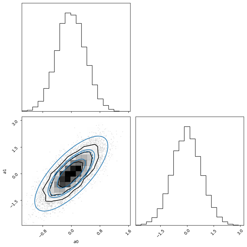
Here we play with a multi-normal distribution.
import corner
from scipy.stats import chi2

rng = np.random.default_rng(seed=2)
L = rng.random((2, 2))
C = L @ L.T

X = rng.multivariate_normal(mean=[0, 0], cov=C, size=10000)
a0, a1 = X.T

dchi2 = np.einsum('ai,aj,ij->a', X, X, np.linalg.inv(C))

fig = plt.figure(figsize=(10,10))
fig = corner.corner(X, fig=fig);
axs = np.array([[fig.axes[0], fig.axes[1]],
                [fig.axes[2], fig.axes[3]]])
ax = axs[1,1]
corner_plot([0, 0], C, axs=axs, labels=['a0', 'a1']);

#ax.plot(chi2.ppf(0.683, df=1), 0, 1, color='y')
chi2s = np.linspace(0, 10, 100)
plt.hist(dchi2, bins=100, density=True);
plt.plot(chi2s, chi2.pdf(chi2s, df=2))
plt.vlines(chi2.ppf([0.683, 0.90, 0.9545, 0.99, 0.9973, 0.9999], df=2), 0, 1, color='y')
<matplotlib.collections.LineCollection at 0x7562f6ec8f50>
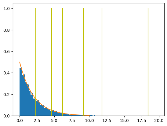
chi2.ppf(0.683, df=2) # Value of chi^2 with ellipse containing 68.3% of the data
np.float64(2.2977070102097144)
a
array([1.25423761, 1.20066782, 3.41499784, 5.61299667])
Confidence Region#
To describe the
If our errors are indeed gaussian and the model is a good fit, then we can consider the parameters \(\vect{a}\) to be distributed with a multivariate normal distribution about their mean \(\bar{\vect{a}}\):
Consider \(\chi^2(\vect{a})\) as a function of the parameters \(\vect{a} = \bar{\vect{a}} + \delta\vect{a}\) where \(\bar{\vect{a}}\) are the exact parameter values for the model with experimental errors \(e_n\) of a known distribution:
If the errors are sufficiently small we can expand the model about the exact parameters in powers of \(\delta\vect{a} = \vect{a} - \bar{\vect{a}}\):
Confidence Levels
If the experimental errors \(e_n\) are independent and normally distributed, and your model is sufficiently linear, then you can use the formulae discussed in section 15.6.5 of [Press et al., 2007] to determine the confidence limits of your parameter estimates and the corresponding covariance matrix \(\mat{C}\). The procedure in this case is:
Let \(\nu\) be the number of fitted parameters whose
If we treat the errors \(e_n\) as independent random variables with distribution \(P_n(e)\), then we can consider the \(\chi^2\) as a random variable:
Consider taking many measurements and averaging. Each measurement will give data \(\{(x_n, y_n)\}\) with a different realization of the errors \(e_n\) sampled from whatever distribution is relevant for the experiment. The resulting \(\chi^2\) will thus have the following distribution The
for some
In the previous section, we computed the best fit parameters \(\bar{\vect{a}}\), and estimated the covariance matrix \(\mat{C}\).
From the least_squares and minimize models, we see that \(\chi^2_r\)
depends on the parameters as:
Extensions#
One can extend this discussion in several ways. For example:
What happens if the errors depend on the parameters?
\[\begin{gather*} y_n = f(x_n; \vect{a}) + e_n(x_n; \vect{a}) \end{gather*}\]What about if the model gives a relationship between \(x_n\) and \(y_n\), but that each has its own errors?
\[\begin{gather*} y_n - e^{(y)}_n = f(x_n - e^{(x)}_n; \vect{a}). \end{gather*}\]This is discussed in section 15.3 of [Press et al., 2007].
References#
Samples, samples, everywhere…: A nice overview of different MCMC software accessible with python.