import mmf_setup;mmf_setup.nbinit()
import logging;logging.getLogger('matplotlib').setLevel(logging.CRITICAL)
%matplotlib inline
import numpy as np, matplotlib.pyplot as plt
This cell adds /home/docs/checkouts/readthedocs.org/user_builds/wsu-phys-581-computation/checkouts/latest/src to your path, and contains some definitions for equations and some CSS for styling the notebook. If things look a bit strange, please try the following:
- Choose "Trust Notebook" from the "File" menu.
- Re-execute this cell.
- Reload the notebook.
Chebyshev Bases#
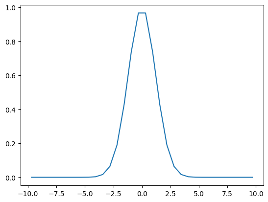
For testing, we will use a Gaussian.
def get_f(x, d=0, x0=0.0, sigma=1.2):
    """Return a gaussian or its derivatives."""
    f = np.exp(-((x-x0)/sigma)**2/2)
    if d == 0:
        return f
    elif d == 1:
        return (x0-x)/sigma**2 * f
    elif d == 2:
        return ((x0-x)**2 - sigma**2)/sigma**4 * f
    else:
        raise NotImplementedError
Fourier Basis#
We start by reviewing how derivatives are computed using the Fourier basis, where we can
represent periodic functions on \(N\) equally spaced points in a box of length \(L\) with
spacing \(h = L/N\) (dx in the code):
(The wavevectors \(k_m\) should be interpreted modulo \(2\pi\) and wrapped so that they extend from \(-\pi/L\). See the code below. On the grid, these values are correct because of aliasing, but should not be used for derivatives. The ordering of \(m\) goes from \(0\) to \(N/2-1\), then from \(-N/2\) back up to \(-1\). See the
code below for a precise specification. (Practically, use numpy.fft.fftfreq().))
These are used to represent a function \(f(x)\) in the box \(-L/2 \leq x < L/2\), and are orthonormal under the following inner product:
N = 32
L = 20.0
dx = L/N
x = np.arange(N) * dx - L / 2
k = 2*np.pi * np.fft.fftfreq(N, dx)
k_ = 2*np.pi * ((N//2 + np.arange(N)) % N - N//2) / L
assert np.allclose(k, k_)
# Basis vectors: Note, the np.fft assumes that the
# abscissa go from 0 to L, so we need to include the -L/2
# shift as a phase
U = np.exp(1j*(x[:, None] + L / 2) * k[None, :])/np.sqrt(N)
assert np.allclose(U.T.conj() @ U, np.eye(N))
# Derivative operators
def get_D(d=1):
"""Return the matrix implementing the d'th derivative."""
return (U * ((1j*k)**d)[None, :]) @ U.T.conj()
def D(f, d=1):
"""Return the `d`'th derivative of `f`."""
coeff = (1j*k)**d
if d % 2 == 1:
coeff[N//2] = 0
return np.fft.ifft(coeff*np.fft.fft(f))
f_x = get_f(x)
# Check that the basis does the FFT. In the FFT, the normalization
# is only in the inverse transform.
assert np.allclose(np.fft.fft(f_x), U.T.conj() @ f_x * np.sqrt(N))
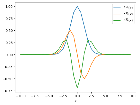
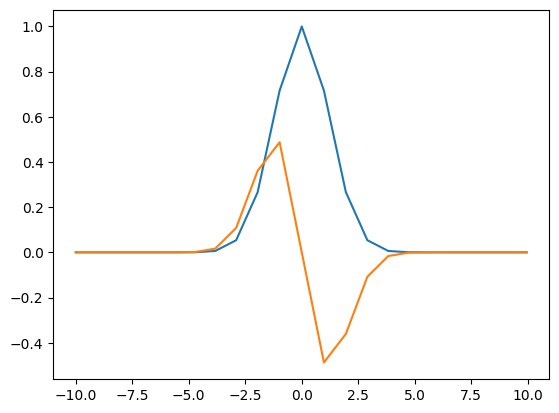
fig, ax = plt.subplots()
for d in [0, 1, 2]:
l, = ax.plot(x, get_f(x, d=d), '-', label=f'$f^{{({d})}}(x)$')
l, = ax.plot(x, D(f_x, d=d).real, ':', c=l.get_c())
assert np.allclose(D(f_x, d=d), get_f(x, d=d), atol=2e-8)
ax.set(xlabel='$x$')
ax.legend()
<matplotlib.legend.Legend at 0x7c7e21ed0c20>
Dirichlet Boundary Conditions#
If you want to impose Dirichlet boundary conditions, use the DST-II transform with endpoints half a grid from the boundary.
These are used to represent a function \(f(x)\) in the box \(-L/2 \leq x < L/2\), and are orthonormal under the following inner product:
Odd Derivatives#
Odd derivatives are a little tricky because the the momenta differ. In particular, the DCT allows \(k_{0} = 0\). Thus, to take the derivative, we must shift the coefficients before calling the DCT (dropping the highest frequency component from the DST).
# Find the fastest way of shifting and dropping.
x = np.random.random(64)

def p1(x):
    res = np.roll(x, 1)
    res[0] = 0
    return res

def p2(x):
    res = np.zeros_like(x)
    res[1:] = x[:-1]
    return res

def p3(x):
    res = np.concatenate([[0], x[:-1]])
    return res


assert np.allclose(p1(x), p2(x))
assert np.allclose(p1(x), p3(x))
%timeit p1(x)
%timeit p2(x)
%timeit p3(x)
5.75 μs ± 67.5 ns per loop (mean ± std. dev. of 7 runs, 100,000 loops each)
1.51 μs ± 3.27 ns per loop (mean ± std. dev. of 7 runs, 1,000,000 loops each)
1.24 μs ± 3.44 ns per loop (mean ± std. dev. of 7 runs, 1,000,000 loops each)
N = 32
L = 20.0
dx = L/N
x = np.arange(N) * dx - L/2 + dx / 2
k = np.pi * (np.arange(N) + 1) / L

def D(f, d=1):
    """Return the `d`'th derivative of `f`."""
    f_k = sp.fft.dst(f, type=2)
    coeff = (-1)**(d // 2) * k ** d
    c_f_k = coeff * f_k
    if d % 2 == 0:
        return sp.fft.idst(c_f_k, type=2)
    else:
        _c = np.concatenate([[0], c_f_k[:-1]])
        return sp.fft.idct(_c, type=2)


f_x = get_f(x)

fig, ax = plt.subplots()
for d in [0, 1, 2]:
    l, = ax.plot(x, get_f(x, d=d), label=f'$f^{{({d})}}(x)$')
    l, = ax.plot(x, D(f_x, d=d), ':', c=l.get_c())
    #print(abs(D(f_x, d=d) -  get_f(x, d=d)).max())
    assert np.allclose(D(f_x, d=d), get_f(x, d=d), atol=1e-8)
ax.set(xlabel='$x$')
ax.legend()
---------------------------------------------------------------------------
NameError                                 Traceback (most recent call last)
Cell In[5], line 24
     22 for d in [0, 1, 2]:
     23     l, = ax.plot(x, get_f(x, d=d), label=f'$f^{{({d})}}(x)$')
---> 24     l, = ax.plot(x, D(f_x, d=d), ':', c=l.get_c())
     25     #print(abs(D(f_x, d=d) -  get_f(x, d=d)).max())
     26     assert np.allclose(D(f_x, d=d), get_f(x, d=d), atol=1e-8)

Cell In[5], line 9, in D(f, d)
      7 def D(f, d=1):
      8     """Return the `d`'th derivative of `f`."""
----> 9     f_k = sp.fft.dst(f, type=2)
     10     coeff = (-1)**(d // 2) * k ** d
     11     c_f_k = coeff * f_k

NameError: name 'sp' is not defined
Chebyshev Basis (Incomplete)#
In particular, we can define this basis on angles \(\theta \in [0, \pi)\) by choosing \(L = \pi\) and shifting by \(\d{\theta}/2\) so that we avoid the endpoints.
The idea of Chebyshev basis is to use the Fourier basis, but on the transformed abscissa
Hence, to compute the derivative of \(f(x)\), we use the FFT to compute the derivative of \(f(\theta)\) as above, then transform back with the chain rule:
The basis vectors are thus
Although this approach works, a problem is that the matrix corresponding to the derivative operator is not anti-Hermitian. To fix this, we look for an alternative proceedure $\( \diff{f(x)}{x} = \diff{f(\theta)}{\theta}\diff{\theta}{x} = f'(\theta)\frac{2}{L \sin \theta}\\ \)$
N = 3
L = 20.0
L_theta = np.pi
d_theta = L_theta / N
theta = np.arange(N) * d_theta + d_theta / 2
x = -L/2 * np.cos(theta)
k_theta = 2*np.pi * np.fft.fftfreq(N, d_theta)
U_theta = np.exp(1j*(theta[:, None] - d_theta / 2) * k_theta[None, :])/np.sqrt(N)
def D(f, d=1):
assert d == 1
coeff = (1j*k_theta)**d
df_dtheta = np.fft.ifft(coeff*np.fft.fft(f))
df_dx = 2/L * df_dtheta / np.sin(theta)
return df_dx
# Derivative operators
def get_D(d=1):
"""Return the matrix implementing the d'th derivative."""
assert d == 1
a = np.sqrt(2 / (L * np.sin(theta)))
b = np.cos(theta) / (L * np.sin(theta))**2
U = a[:, None] * U_theta
D_k = ((1j*k_theta)**d)
return ((a**2)[:, None] * U_theta * D_k[None, :]) @ U_theta.T.conj()
return (U * D_k[None, :]) @ U.T.conj() - np.diag(b)
#assert np.allclose(D(f_x, d=1), get_D(d=1) @ f_x)
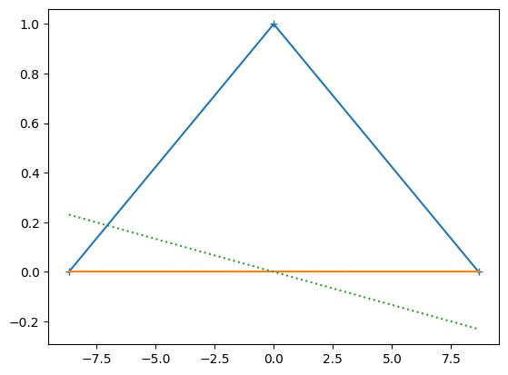
f_x = get_f(x, d=0)
plt.plot(x, f_x, '-+')
plt.plot(x, get_f(x, d=1), '-')
plt.plot(x, D(f_x, d=1), ':')
print(abs(D(f_x, d=1) - get_D(d=1) @ f_x).max())
1.665358527103748e-16
/home/docs/checkouts/readthedocs.org/user_builds/wsu-phys-581-computation/conda/latest/lib/python3.13/site-packages/matplotlib/cbook.py:1719: ComplexWarning: Casting complex values to real discards the imaginary part
  return math.isfinite(val)
/home/docs/checkouts/readthedocs.org/user_builds/wsu-phys-581-computation/conda/latest/lib/python3.13/site-packages/matplotlib/cbook.py:1355: ComplexWarning: Casting complex values to real discards the imaginary part
  return np.asarray(x, float)
D1 = get_D(d=1)
abs(D1 + D1.T.conj()).max()
np.float64(0.1154700538379252)
N = 32
L = 20.0

L_theta = np.pi
d_theta = L_theta / N
theta = np.arange(N) * d_theta
x = -L/2 * np.cos(theta)
k_theta = 2*np.pi * np.fft.fftfreq(N, d_theta)

U_theta = np.exp(1j*(theta[:, None]) * k_theta[None, :])/np.sqrt(N)
assert np.allclose(U.T.conj() @ U, np.eye(N))

# Derivative operators
def get_D(d=1):
    """Return the matrix implementing the d'th derivative."""
    return (U * ((1j*k)**d)[:, None]) @ U.T.conj()


def get_f(x, d=0, x0=0.0, sigma=1.2):
    """Return a gaussian or its derivatives."""
    f = np.exp(-((x-x0)/sigma)**2/2)
    if d == 0:
        return f
    elif d == 1:
        return (x0-x)/sigma**2 * f
    elif d == 2:
        return ((x0-x)**2 - sigma**2)/sigma**4 * f
    else:
       raise NotImplementedError


def D(f, d=1):
    """Return the `d`'th derivative of `f`."""
    coeff = (1j*k)**d
    return np.fft.ifft(coeff*np.fft.fft(f))

f_x = get_f(x)

# Check that the basis does the FFT.  In the FFT, the normalization
# is only in the inverse transform.
assert np.allclose(np.fft.fft(f_x), U.T.conj() @ f_x * np.sqrt(N))

fig, ax = plt.subplots()
for d in [0, 1, 2]:
    l, = ax.plot(x, get_f(x, d=d), label=f'$f^{{({d})}}(x)$')
    assert np.allclose(D(f_x, d=d), get_f(x, d=d), atol=2e-8)
ax.set(xlabel='$x$')
ax.legend()
---------------------------------------------------------------------------
AssertionError                            Traceback (most recent call last)
Cell In[8], line 46
     44 for d in [0, 1, 2]:
     45     l, = ax.plot(x, get_f(x, d=d), label=f'$f^{{({d})}}(x)$')
---> 46     assert np.allclose(D(f_x, d=d), get_f(x, d=d), atol=2e-8)
     47 ax.set(xlabel='$x$')
     48 ax.legend()

AssertionError:
Trefethan#
Here is an implementation of the formula provided by Trefethen:
def get_x_D(N):
"""Return `(x, D)`, the points and derivative matrix."""
if N == 1:
x = np.array([1])
D = np.array([[0]])
return x, D
theta = np.pi * np.arange(N)/(N-1)
x = np.cos(theta)
c = np.ones(N)
c[0] = c[-1] = 2.0
c = c[:, np.newaxis] * (-1) ** np.arange(N)
dX = x[:, None] - x[None, :]
D = c/c.T / (dX + np.eye(N))
D -= np.diag(D.sum(axis=-1))
return x, D
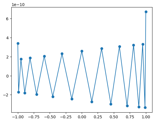
x, D = get_x_D(21)
f_x = np.exp(x)*np.sin(5*x)
df_x = np.exp(x)*(np.sin(5*x) + 5*np.cos(5*x))
plt.plot(x, D@f_x - df_x, '-o')
[<matplotlib.lines.Line2D at 0x7c7e20f29e50>]