Fourier Techniques

Fourier Techniques#

The idea behind Fourier techniques is to express a signal \(f(x)\) in terms of a series of sine waves, or often more conveniently, in terms of plane waves \(\exp(\I k x)\):

\[\begin{gather*} f(x) = \sum_{k} \tilde{f}_{k}e^{\I k x}, \qquad e^{\I k x} = \cos(kx) + \I \sin(kx). \end{gather*}\]

The coefficients \(\tilde{f}_{k}\) are called the Fourier coefficients, and the role of the Fourier transform is to compute these.

Exactly what this means depends on the context, which determines which values of \(k\) appear in the preceding expressions. Some common cases include:

Fourier Transform: The most general expression for a function \(f(x): \mathbb{R}\rightarrow \mathbb{C}\) is the continuous Fourier transform:

\[\begin{gather*} \newcommand{\F}{\mathcal{F}} \overbrace{ f(x) = \underbrace{ \int_{-\infty}^{\infty} \frac{\d{k}}{2\pi}\; \tilde{f}_{k} e^{\I k x} }_{\text{Inverse Fourier transform}}}^{f = \F^{-1}(\tilde{f}),} \qquad \overbrace{ \tilde{f}_{k} = \underbrace{ \int_{-\infty}^{\infty} \d{x}\; e^{-\I k x} f(x) }_{\text{Fourier transform}}}^{\tilde{f} = \F(f).} \end{gather*}\]

This can be used to express the completeness relationship in terms of the following integrals:

\[\begin{gather*} \int_{-\infty}^{\infty}\d{x}\; e^{\I (k-q) x} = 2\pi \delta(k-q),\\ \int_{-\infty}^{\infty}\frac{\d{k}}{2\pi}\; e^{\I k (x-y)} = \delta(x-y). \end{gather*}\]

The key for this is the following completeness relationship:

\[\begin{gather*} \int_{-\infty}^{\infty}\d{x}\; e^{\I k x} = 2\pi \delta(k). \end{gather*}\]

where \(\delta(x)\) is the Dirac delta function.
Fourier Series: For strictly periodic functions \(f(x+L) = f(x)\), we must choose \(k\) so that the basis functions are periodic.

\[\begin{gather*} e^{\I k (x + L)} = e^{\I k x}e^{\I k L} = e^{\I k x}, \qquad k_n = \frac{2\pi n}{L}. \end{gather*}\]

Hence, the \(k\)s take on discrete values and the function \(f(x)\) can be expressed in terms of a Fourier series:

\[\begin{gather*} f(x) = \sum_{n=-\infty}^{\infty} \tilde{f}_{k_n} e^{\I k_n x}. \end{gather*}\]

The corresponding completeness relationship is

\[\begin{gather*} \sum_{n=-\infty}^{\infty} e^{\I k_n x} = \sum_{m=-\infty}^{\infty} \delta(x - mL) \equiv Ш_{L}(x). \end{gather*}\]

The right-hand side here is sometimes known as a Dirac comb.
Discrete Fourier Transform: If we further restrict our attention to functions sampled on a set of lattice of points \(x_m = x_0 + m \delta\) with lattice space \(\delta = L/N\), then we can restrict the number of Fourier modes to be finite:

\[\begin{gather*} f(x_m) = \sum_{n=0}^{N-1} \tilde{f}_{k_n} e^{\I k_n x_m}. \end{gather*}\]

This is “obvious” if you think of \(e^{\I \theta}\) as unit vectors in the complex plane. This sums over a set of vectors that completely cancels unless the exponent is zero, in which case they all point in the same direction.

The key for this is the following completeness relationship:

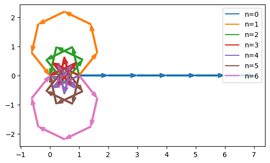
\[\begin{gather*} \frac{1}{N}\sum_{m=0}^{N-1} \exp\left(\frac{2\pi \I n m}{N}\right) = \delta_{n0}, \end{gather*}\]

where \(\delta_{mn}\) is the Kronecker delta. This discrete Fourier transform (DFT) is the domain of computer implementations of the FFT.

N = 7
n = np.arange(N)[:, None]
m = np.arange(N)[None, :]
M = np.exp(2j*np.pi * m * n / N) 
assert np.allclose(M.sum(axis=1)/N, [1, 0, 0, 0, 0, 0, 0])

phasor = np.cumsum(M, axis=1)
fig, ax = plt.subplots()
for n in range(N):
    z = phasor[n]
    ax.plot(z.real, z.imag, label=f"{n=}")
    for z0, z1 in zip(z[:-1], z[1:]):
        dz = z1 - z0
        ax.arrow(z0.real, z0.imag, dz.real, dz.imag, width=0.05,
        length_includes_head=True, fc=f"C{n}", ec=f"C{n}")
ax.set(aspect=1)
ax.legend(loc='upper right');

../_images/d4f79af8ba238990226c7ff90ea953b9c52e787badb3380342f38bb997182760.png

A Unified Approach#

I recommend considering the \(N\)-point discrete Fourier transform as the base case, and then taking the appropriate continuum (\(N\rightarrow \infty\)) or thermodynamic (\(L \rightarrow \infty\)) limits:

\[\begin{gather*} n \in \{0, 1, \cdots, N-1\},\\ \begin{aligned} x_{n} &= n \d{x} \in [0, L) \mod L, & \d{x} &= \frac{L}{N},\\ k_{n} &= n\d{k} \in \Bigl[-\frac{\pi}{\d{x}}, \frac{\pi}{\d{x}}\Bigr) \mod \frac{2\pi}{\d{x}}, & \d{k} &= \frac{2\pi}{L}. \end{aligned} \end{gather*}\]

Here the momenta \(k_n\) shifted by appropriate factors of \(2\pi/L\) to lie in the interval \([-\pi/\d{x}, \pi/\d{x})\). Thus, numerically, the values of the frequencies \(f_n\) returned by numpy.fft.fftfreq() for example are given by the code

f_n = ((np.arange(N) / N + 0.5) % 1 - 0.5)/dx

With these definitions, we can define the continuum version by taking \(N\rightarrow \infty\) and/or \(L\rightarrow \infty\) while taking

\[\begin{align*} \d{x}\sum_{n} = \frac{L}{N}\sum_{n} &\rightarrow \int \d{x}, \\ \d{k}\sum_{n} = \frac{2\pi}{L}\sum_{n} &\rightarrow \int \d{k}, \\ \delta_{mn}/\d{x} &\rightarrow \delta(x_m -x_n),\\ \delta_{mn}/\d{k} &\rightarrow \delta(k_m - k_n). \end{align*}\]

I generally like to keep my factors of \(2\pi\) with my momentum integrals and momentum delta-functions, so I also use

\[\begin{align*} \frac{1}{L}\sum_{n} &\rightarrow \int \frac{\d{k}}{2\pi}, & L\delta_{mn} &\rightarrow 2\pi\delta(k_m - k_n). \end{align*}\]

The completeness relationship follows from:

\[\begin{align*} \frac{1}{N}\sum_{n=0}^{N-1} e^{\overbrace{2\pi \I mn/N}^{\I k_m x_n}} &= \delta_{m0},\\ \underbrace{\frac{L}{N}}_{\d{x}}\sum_{n=0}^{N-1} e^{\I x_n k_m} \rightarrow \int \d{x}\; e^{\I x k_m} &= 2\pi \delta(k_m) \leftarrow L\delta_{m0},\\ \underbrace{\frac{1}{L}}_{\d{k}/2\pi}\sum_{n=0}^{N-1} e^{\I x_n k_m} \rightarrow \int \frac{\d{k}}{2\pi}\; e^{\I x k_m} &= \delta(x_m) \leftarrow \frac{\delta_{m0}}{\d{x}},\\ \end{align*}\]

The Fast Fourier Transform (FFT).

The discovery of the Fast Fourier Transform (FFT) algorithm revolutionized many computational techniques by dropping the cost of computing the discrete Fourier transform from \(\order(N^2)\) to \(\order(N\log N)\). Current implementations (see the FFTw) keep the prefactor small, making FFT-based techniques preferred wherever applicable. In particular, the FFT has efficient implementations, both on CPUs and on hardware accelerators like GPUs. Thus, if the computational cost of an algorithm is dominated by the DFT, then these algorithms can be implemented almost as efficiently in a high-level language like Python as in a low-level, high-performance language like C++ or Fortran.

Derivatives#

One of the primary uses of Fourier techniques is to compute derivatives:

\[\begin{align*} f(x) &= \sum_{n} \tilde{f}_{k_n} e^{\I k_n x},\\ f'(x) &= \sum_{n} \I k_n \tilde{f}_{k_n} e^{\I k_n x},\\ f''(x) &= \sum_{n} -k_n^2 \tilde{f}_{k_n} e^{\I k_n x},\\ f^{(d)}(x) &= \sum_{n} (\I k_n)^d \tilde{f}_{k_n} e^{\I k_n x},\\ \end{align*}\]

Thus, “in Fourier space”, we have:

\[\begin{gather*} \diff{}{x} \equiv \I k \end{gather*}\]

in the sense that the Fourier coefficients are multiplied by this factor \(\tilde{f}_k \rightarrow \I k \tilde{f}_k\).

Warning

The factor of \(\I = \sqrt{-1}\) in the odd derivatives can cause unexpected behavior if the number of lattice points is even. These stem from the fact that there is only one \(k=0\) momentum, while all others are paired \(\pm 2\pi n/L\). If the number of lattice points is even, there must therefore be an unpaired finite momentum. This turns out to be \(k_{N/2} = \pi N /L\), the momentum with highest magnitude in the space, corresponding to alternations between even and odd lattice.

The subtle issue is that, if your function has any component with this momentum, then the derivative will be complex, even if your function is real. This is common if your function contains any sharp features, as these will contain high-momentum components.

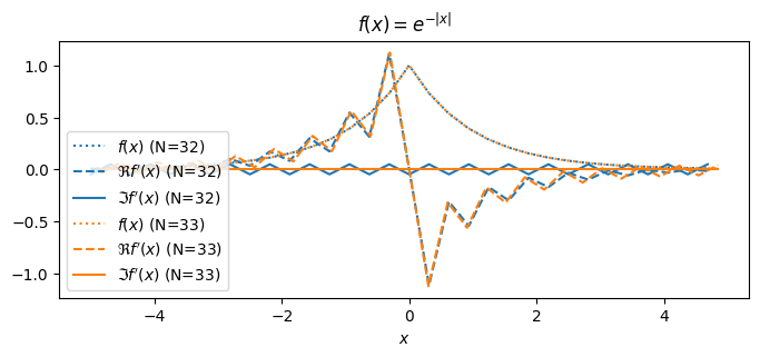
../_images/57f61b67e1a9f4a6ed4b82ecf35a2535e9ac206dd350cdcb5dbd24cc900392d1.png — Fig. 1 Derivative of a sharply kinked function with an even and odd number of lattice points. Notice that with an even number of points there is a sizable imaginary component to the derivative \(f'(x)\), even though the original function is real.#

One way to mitigate this is to set this component to zero when computing the derivative with code like k[N//2] = 0, but this has consequences. For example, with denoising, doing this will prevent the code from being able to remove the highest-frequency noise, which might be exactly what one is trying to do!

We used this in our code to quickly implement the Laplacian operator for images

\[\begin{gather*} \nabla^2 = \pdiff[2]{}{x} + \pdiff[2]{}{y}: \end{gather*}\]

def laplacian(f, dx=1.0):
    """Return the Laplacian of f."""
    
    # If f.shape is fixed, K2 could be precomputed for speed
    Nx, Ny = f.shape
    Lx, Ly = dx*Nx, dx*Ny
    kx, ky = [2*np.pi * np.fft.fftfreq(_N, dx) for _N in (Nx, Ny)]
    
    # x goes down (first index), y goes across (second index)
    kx, ky = kx[:, np.newaxis], ky[np.newaxis, :]
    
    K2 = kx**2 + ky**2
    
    return np.fft.ifftn(-K2 * np.fft.fftn(f))

from scipy.ndimage import laplace
from phys_581 import denoise
im = denoise.Image()
f = im.get_data()
d2f = laplace(f, mode='wrap')
d2f_fft = laplacian(f)
assert np.allclose(d2f_fft.imag, 0)
d2f_fft = d2f_fft.real

rel_err = abs(d2f_fft - d2f).mean() / abs(d2f).mean()
print(f"{rel_err=:.2g}")

fig, axs = denoise.subplots(2)
im.show(d2f, vmin=-0.1, vmax=0.1, ax=axs[0])
axs[0].set(title="Finite Difference")
im.show(d2f_fft, vmin=-0.1, vmax=0.1, ax=axs[1])
axs[1].set(title="FFT");

---------------------------------------------------------------------------
ImportError                               Traceback (most recent call last)
Cell In[6], line 2
      1 from scipy.ndimage import laplace
----> 2 from phys_581 import denoise
      3 im = denoise.Image()
      4 f = im.get_data()

ImportError: cannot import name 'denoise' from 'phys_581' (/home/docs/checkouts/readthedocs.org/user_builds/wsu-phys-581-computation/checkouts/latest/src/phys_581/__init__.py)

Although these look quite similar, the actual error is large in places because the function scipy.ndimage.laplace() uses a finite difference approximation with a 3-point stencil:

\[\begin{gather*} f''(x) \approx \frac{f(x-h) - 2f(x) + f(x+h)}{h^2} = D_2[f](x). \end{gather*}\]

To understand the precise nature of the difference between this an the FFT method, we can also apply a Fourier technique:

\[\begin{align*} D_2[f] &= \sum_{n} \tilde{f}_{k_n} \frac{ \overbrace{ e^{\I k_n (x-h)} - 2e^{\I k_n x} + e^{\I k_n (x+h)} }^{e^{\I k_n x}(e^{-\I k_n h} - 2 + e^{\I k_n h})} }{h^2} = \sum_{n} \tilde{f}_{k_n} e^{\I k_n x} 2\frac{ \overbrace{\cos(k_n h) - 1}^{\frac{(k_n h)^2}{2!} - \frac{(k_n h)^4}{4!} + \cdots} }{h^2}\\ &= \sum_{n} \tilde{f}_{k_n} e^{\I k_n x} \left( -k_n^2 +\frac{k_n^4 h^2}{12} + \order(h^4) \right). \end{align*}\]

Thus, we see that the finite difference approximation has the same \(-k^2\) term, but contains additional terms that vanish in the \(h\rightarrow 0\) limit. In our case, \(h=1\), \(L\approx N \approx 500\), and so the maximum momentum is \(k_\max \approx \pi\). We expect the relative error to thus be

\[\begin{gather*} \frac{k_\max^2 h^2}{12} \approx \frac{\pi^2}{12} \approx 0.8, \end{gather*}\]

consistent with the numerical value. If the image were smooth, then \(k_\max\) would be smaller than this, reducing the error, but, since there are sharp features, the relative error here is large.

def laplacian2(f, dx=1.0):
    """Return the Laplacian of f using the cos() dispersion."""
    Nx, Ny = f.shape
    Lx, Ly = dx*Nx, dx*Ny
    kx, ky = [2*np.pi * np.fft.fftfreq(_N, dx) for _N in (Nx, Ny)]
    kx, ky = kx[:, np.newaxis], ky[np.newaxis, :]
    h = dx
    K2 = -2 * ((np.cos(kx*h) - 1) + (np.cos(ky*h) - 1)) / h**2
    
    return np.fft.ifftn(-K2 * np.fft.fftn(f))

from scipy.ndimage import laplace
from phys_581 import denoise
d2f_fft = laplacian2(f)
assert np.allclose(d2f_fft.imag, 0)
d2f_fft = d2f_fft.real

rel_err = abs(d2f_fft - d2f).mean() / abs(d2f).mean()
print(f"{rel_err=:.2g}")

---------------------------------------------------------------------------
ImportError                               Traceback (most recent call last)
Cell In[7], line 13
     10     return np.fft.ifftn(-K2 * np.fft.fftn(f))
     12 from scipy.ndimage import laplace
---> 13 from phys_581 import denoise
     14 d2f_fft = laplacian2(f)
     15 assert np.allclose(d2f_fft.imag, 0)

ImportError: cannot import name 'denoise' from 'phys_581' (/home/docs/checkouts/readthedocs.org/user_builds/wsu-phys-581-computation/checkouts/latest/src/phys_581/__init__.py)

From this tiny error – on the order of the machine precision – we see that these are indeed equivalent.

The Connection with Renormalization Group

The picture here is closely related to the Renormalization Group. In Fourier space, there are infinitely many different forms of the second derivative operator

\[\begin{gather*} \diff[2]{}{x} \equiv -k^2 + c_2 hk^3 + c_4 h^2k^4 + \cdots, \end{gather*}\]

where the coefficients \(c_n\) are dimensionless. As one “coarse grains”, taking the lattice spacing \(h \rightarrow 0\), all of these different derivative operators approach the same continuum result. This requires that the momenta \(k\) be bounded: i.e. that there is some smallest natural length scale \(\xi\) below which \(h \ll \xi\) the physics does not change. This is the so-called “continuum limit”, and any sensible computational model should have a well-defined limit.

In this case, the image or signal is often characterized by an analytic function – functions whose power-series converges everywhere – and the Fourier technique gives exponential accuracy.

Approximations with exponential convergence like this are often called spectral methods (see [Boyd, 1989]), and discretization methods will often add correction terms to improve convergence. In this sense, the Fourier approach with just the \(-k^2\) term may be considered “the best”, but it is far from clear that this is “the best” from a computational perspective.

For example, an image might actually have sharp features. These will not be described by analytic functions, and spectral methods will be no better than finite-difference techniques, with power-law convergence. Finite-difference techniques can have an advantage in these cases, minimizing ringing artifacts, for example. Don’t immediately give up on less-accurate approximations unless you know something about the smoothness of your signals.

Convolution and Toeplitz Matrices#

In the previous section, we saw that Fourier techniques allowed us to obtain a spectral representation of the derivative, and to understand how the finite difference formula behaves. The reason this works is because these operations behave as a convolution in real space, which becomes multiplication in Fourier space:

\[\begin{gather*} (f*g)(x) = \int_{-\infty}^{\infty} f(x-z)g(z)\d{z},\qquad \F(f*g) = \F(f)\F(g). \end{gather*}\]

The convolution, in turn, is simply matrix multiplication by a matrix whose entries depend only on the distance from the diagonal – so-called Toeplitz matrices. Finite-difference matrices have this form (with appropriate boundary conditions – periodic as shown, or Dirichlet):

\[\begin{gather*} \mat{D}_2 = \frac{1}{\d{x}^2} \begin{pmatrix} -2 & 1 & & & 1\\ 1 & -2 & 1 \\ & 1 & \ddots & \ddots\\ & & \ddots & -2 & 1\\ 1 & & & 1 & -2. \end{pmatrix}. \end{gather*}\]

To compute the derivative, take the Fourier transform of your function, multiply by the Fourier transform of the Toeplitz matrix, and then take the inverse transform:

\[\begin{gather*} f'(x) \approx \underbrace{\F^{-1}\Bigl(-k^2 \F(f)\Bigr)}_{\text{Fourier}} \approx \underbrace{ \F^{-1}\Bigl(2(\cos k - 1)\F(f)\Bigr) }_{\text{finite difference}}, \end{gather*}\]

etc.

If your signal processing algorithm can be expressed as a Toeplitz matrix, then Fourier techniques provide a simple way of exactly solving the problem (up to round-off errors) as the matrix will be diagonal in Fourier space.

Product rule#

It is important to note that the product rule – an important mathematical identity – generally does not hold for numerical derivative techniques. Specifically, for two functions \(f(x)\) and \(g(x)\), while

\[\begin{gather*} \diff{f(x)g(x)}{x} = f'(x)g(x) + f(x) g'(x), \end{gather*}\]

the corresponding case does not hold numerically:

\[\begin{gather*} D(fg) \approx D(f)g + fD(g). \end{gather*}\]

While this should approximately hold for smooth functions, it will almost always have errors for functions with sharp boundaries. To see this, consider a matrix representation:

\[\begin{gather*} [D(f)]_{i} = \sum_j D_{ij}f_j, \qquad [D(fg)]_i = \sum_j D_{ij}f_jg_j, \\ [D(f)g + fD(g))]_i = \sum_j D_{ij}(f_jg_i + f_ig_j). \end{gather*}\]

Now consider \(f_i = \delta_{ia}\) and let \(g'_i \equiv [D(g)]_i\). Then, if the product rule was exactly satisfied, we would have

\[\begin{gather*} D_{ia}g_a = D_{ia}g_i + \delta_{ai}g'_i. \end{gather*}\]

This says that, if \(i=a\), then \(g'_a = 0\): hence the relationship can only be exactly true if \(g\) must be a constant.

Care must be employed when using the product rule in finite manipulations, especially integration by parts. Thus, while the following is correct in the continuum limit (up to boundary terms which vanish for periodic, Dirichlet, or Neumann boundary conditions):

\[\begin{gather*} E[u] = \int\frac{1}{2}\abs{\vect{\nabla}u}^2 + \frac{\lambda}{2}\int\abs{u - d}^2,\qquad E'[u] = -\nabla^2u + \lambda(u - d), \end{gather*}\]

it is not exact for finite computations.

Instead, if trying to implement this with a minimize that requires high-accurate derivatives, make sure that the energy is computed in a way that exactly defines the appropriate minimization problem such as in the following case:

\[\begin{gather*} E[u] = \int\frac{-u\nabla^2 u}{2} + \frac{\lambda}{2}\int\abs{u - d}^2. \end{gather*}\]

While this is formally equivalent in the continuum limit, it is also exactly equivalent numerically to the numerical implementation of \(E'[u]\) as long as the matrix representing \(\mat{D}_2 \approx \nabla^2\) is symmetric \(\mat{D}_s^T = \mat{D}_2\).

Exercises#

Exploring the DFT#

Consider a function in 1D \(f(x)\) tabulated on \(N\) lattice points \(x_n = n\d{x}\) in a periodic box of length \(L = N \d{x}\). As a test function, consider:

\[\begin{align*} f_{\eta}(x) &= \exp\left(\frac{-1}{1+\eta\cos(k x)}\right),\\ f'_{\eta}(x) &= \frac{-\eta k \sin(k x)}{\bigl(1+\eta\cos(k x)\bigr)^2}f_{\eta}(x),\\ f''_{\eta}(x) &= \frac{-\eta k^2\Bigl(\eta\bigl(1 + \cos^2(kx) - \eta\cos^3(kx)\bigr) + (1+2\eta^2)\cos(kx)\Bigr)}{\bigl(1+\eta\cos(k x)\bigr)^4} f_{\eta}(x) \end{align*}\]

where \(k = 2\pi n/L\) is one of the lattice momenta to ensure that the function has appropriate periodicity:

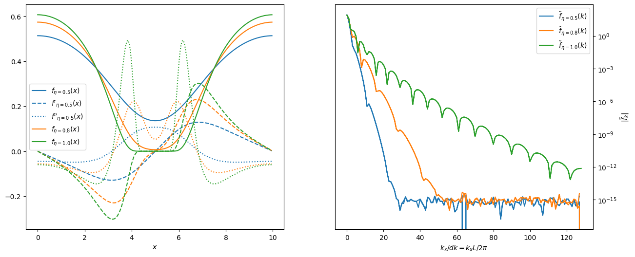
../_images/32f2397ea7efb69342191142a66a715a9ab151d5b1ad00110c879662717cab1c.png

This function has the property that it is formally analytic for \(\eta < 1\), but becomes non-analytic with essential singularities at \(\cos(kx)=-1\) for \(\eta = 1\):

\[\begin{gather*} f_1(x) = \exp\left(\frac{1}{1+\cos(kx)}\right). \end{gather*}\]

Note, however, that the function remains very smooth \(f_1 \in C^\infty\).

For \(\eta<1\), we see the typical behavior that the magnitude of the Fourier coefficients falls exponentially as a function of the wave-number \(n = k_n/\d{k}\). In this particular case, we expect to achieve machine precision for \(n > 30\) for \(\eta = 0.5\) and for \(n>50\) for \(\eta = 0.8\). This means, that we only need \(N=60\) or \(N=100\) points respectively to accurately represent and work with the function.

Once we lose analyticity, however, then the Fourier coefficients start falling off as a power law, and we need far more points. For smooth functions like this, spectral methods still do better than finite difference, but if there is a cusp or discontinuity, then spectral methods lose their advantage.

Note that the functions \(f_\eta(x)\) are both periodic over \(x\in[0, L]\) and flat at the boundaries, therefore satisfying Neumann boundary conditions. Use the functions to test your code.

Represent the function \(f(x)\) as a vector \(\ket{f}\) that can be expressed in terms of its tabulated values \(f_n = f(x_n)\) in the standard basis \(\{\ket{x_n}\}\):

\[\begin{gather*} \ket{f} = \sum_{n} \ket{x_n}f_n = \sum_{n} \ket{x_n}f(x_n). \end{gather*}\]

Think of this numerically in terms of the column vectors:

\[\begin{gather*} \ket{x_0} = \begin{pmatrix} 1 \\ 0 \\ \vdots\\ 0 \end{pmatrix}, \qquad \ket{x_1} = \begin{pmatrix} 0 \\ 1 \\ \vdots\\ 0 \end{pmatrix},\qquad \ket{f} = \begin{pmatrix} f_0 = f(x_0)\\ f_1 = f(x_1)\\ \vdots\\ f_{N-1} = f(x_{N-1}) \end{pmatrix}. \end{gather*}\]

The standard basis is orthonormal and complete:

\[\begin{gather*} \braket{x_m|x_n} = \delta_{nm}, \qquad \mat{1} = \sum_{n}\ket{x_n}\bra{x_n}, \end{gather*}\]

hence, the first expression is:

\[\begin{gather*} \ket{f} = \mat{1}\ket{f} = \sum_{n}\ket{x_n}\underbrace{\braket{x_n|f}}_{f_n=f(x_n)} = \sum_{n}\ket{x_n}f_n. \end{gather*}\]

The Fourier transform can be simply thought of as a change of basis into a new basis of plane waves \(\{\ket{k_n}\}\) corresponding to the functions \(\exp(\I k_n x)\). To make this all work out, we must properly normalize the vectors:

\[\begin{gather*} \braket{x_m|k_n} = \frac{1}{\sqrt{N}}e^{\I k_n x_m} = [\mat{F}^{-1}]_{mn}. \end{gather*}\]

As we shall show, these are the coefficients of the matrix \(\mat{F}^{-1}\) implementing the inverse Fourier transform.

Exercise: Show that \(\braket{k_i|k_j} = \delta_{ij}\).

\[\begin{gather*} \braket{k_i|k_j} = \braket{k_i|\mat{1}|k_j} = \sum_{n}\overbrace{\braket{k_i|x_n}}^{\frac{e^{-\I k_ix_n}}{\sqrt{N}}} \overbrace{\braket{x_n|k_j}}^{\frac{e^{\I k_jx_n}}{\sqrt{N}}}\\ = \frac{1}{N}\sum_{n}e^{\I (k_j - k_i) x_n} = \frac{1}{N}\sum_{n=0}^{N-1}e^{2\pi \I (j - i) n/N} = \delta_{ij}. \end{gather*}\]

The DFT is the transformation that takes the coefficients \(f_n = \braket{x_n|f}\) into the Fourier coefficients \(\tilde{f}_m = \braket{k_m|f}\). In the standard basis, this can be represented by a matrix \(\mat{F}\) :

\[\begin{gather*} \tilde{f} = \F(f), \qquad \tilde{f}_m = \sum_{n}[\mat{F}]_{mn}f_n. \end{gather*}\]

Exercise: What is the matrix \(\mat{F}\) and its inverse \(\mat{F}^{-1}\)?

Expanding these coefficients, we have

\[\begin{gather*} \overbrace{\braket{k_m|f}}^{\tilde{f}_m} = \sum_{n}[\mat{F}]_{mn}\overbrace{\braket{x_n|f}}^{f_n}. \end{gather*}\]

Inserting \(\mat{1}\) on the left and expanding this using the completeness of the standard basis

\[\begin{gather*} \sum_{n}\braket{k_m|x_n}\braket{x_n|f} = \sum_{n}[\mat{F}]_{mn}\braket{x_n|f} \end{gather*}\]

allows us to identify:

\[\begin{gather*} [\mat{F}]_{mn} = \braket{k_m|x_n} = \braket{x_n|k_m}^* = \frac{e^{-\I k_m x_n}}{\sqrt{N}} = \frac{e^{-2\pi \I mn/N}}{\sqrt{N}}. \end{gather*}\]

This matrix is unitary, hence the inverse is just the conjugate transpose:

\[\begin{gather*} \mat{F}^{-1} = \mat{F}^\dagger, \qquad [\mat{F}^{-1}]_{mn} = [\mat{F}]^{*}_{nm} = \frac{e^{2\pi \I mn/N}}{\sqrt{N}}. \end{gather*}\]

Check these numerically, but note that the numerical implementations have a different normalization:

\[\begin{gather*} [\mat{F}]_{mn} = e^{-2\pi \I mn / N}, \qquad [\mat{F}^{-1}]_{mn} = \frac{1}{N}e^{2\pi \I mn / N}. \end{gather*}\]

I.e. the factor \(1/N\) is included only in the inverse transform. For performance, some implementations (in particular, the FFTw) drop even this factor, leaving it up to the user.

To create these matrices, simply use broadcasting, with the first index going down through the rows, and the second index going across through the columns:

F = np.exp(-2j*k[:, np.newaxis]*x[np.newaxis, :])
Finv = np.exp(2j*k[np.newaxis, :]*x[:, np.newaxis]) / N

I think of this as follows: the second index of F should act on f(x), hence should have changing \(x\) values. Thus, we need x[np.newaxis, :]. The colon here indicates which axis actually changes, while the np.newaxis (older codes use None) represents copied values:

\[\begin{align*} \texttt{x[:, np.newaxis]} = \begin{pmatrix} x_0 \\ % x_1 \\ \vdots\\ x_{N-1} \end{pmatrix} &\equiv \begin{pmatrix} x_0 & x_0 & \cdots\\ % x_1 & x_1 & \cdots\\ \vdots & \vdots\\ x_{N-1} & x_{N-1} & \cdots \end{pmatrix}, \\ \texttt{x[np.newaxis, :]} = \begin{pmatrix} x_0 & \cdots & x_{N-1} \end{pmatrix} &\equiv \begin{pmatrix} x_0 % & x_1 & \cdots & x_{N-1}\\ x_0 %& x_1 & \cdots & x_{N-1}\\ \vdots % & \vdots & & \vdots \end{pmatrix}. \end{align*}\]

The broadcasting in NumPy refers to the behavior that, although these arrays are actually only a single column vector x[:, np.newaxis].shape == (N, 1) and a single row vector x[np.newaxis, :].shape == (1, N) respectively, they will behave in expressions as if they are full matrices as shown, with enough copies to make sense. This can result in significant performance improvements, both for speed, and memory, if used appropriately.

Likewise, the inverse transform satisfies

\[\begin{gather*} f = \F^{-1}(\tilde{f}), \qquad f_n = \sum_{m}[\mat{F}^{-1}]_{nm}\tilde{f}_m. \end{gather*}\]

Exercise: Exploring the DFT.

Use the formulae defined here, and the FFT as implemented in NumPy to compute the derivatives of the provided test function. Compare this with finite-difference approximations and explore how these depend on the number of points used.

Other Applications#

In this document we have focused on the standard complex Fourier transform for periodic functions. There are many other closely related applications, many of which are discussed on the DFT page. For example:

Computing the DFT of purely real and imaginary signals.
The discrete cosine and sine transforms (DCT and DST). These allow you to implement different boundary conditions or deal with even and odd function. For example, the DCT implements a DFT for even functions, while the DST allows you to transform odd functions. There are actually 8 different DST transforms allowing one to consider various mixed boundary conditions (Dirichlet and Neumann). These are simple conceptually, but very tricky in the details: special attention must be paid to about exactly which grid point or interval the function is symmetric about.