Execution Time and Extremal Value Theory#
Consider the problem of measuring the execution time of a small piece of code or a particular machine. There is lower bound – the fastest that code can be executed – but any given measurement is likely to be larger due to other actions performed by the computer (checking email, garbage collection, cache misses etc.). Thus, a reasonable approach to characterizing the performance of that code might be to consider the minimum of a bunch of measurements. Alternatively, one might like to consider the median (50th percentile) or another fixed percentile.
In this note, we will address the question: how many measurements should we make to obtain an accurate representation of the execution time?
Measurement#
Actually measuring execution time is quite complicated due to issues like clock
resolution, quantization errors, synchronization, etc. For some details, see
[Stewart, 2001]. We shall assume that these are accounted for in the following:
in this case, through the timeit module in the Python standard library.
Model#
Our model will be that the measured execution time \(t\) is a random variable with some PDF \(p(t)\). For example:
import timeit
import math
#from mmfutils.plot.histogram import hist_err

Ns = 10000

fig, axs = plt.subplots(1, 3, figsize=(9, 3))

for number, ax in zip([10, 100, 1000], axs):
    tss = np.array([[
            timeit.timeit('math.sin(1.2)', 'import math', number=number)/number
            for n in range(Ns)]
        for n in range(3)])

    t_min = tss.ravel().min()
    factor, unit, t_min = format_time(t_min)
    t0, t1 = np.percentile(tss.ravel() * factor, [0, 99])
    h, dh, bins = histogram_err(tss.ravel()*factor, bins=500)

    plt.sca(ax)
    for ts in tss:
        hist_err(ts*factor, bins=bins, density=True)
    ax.set(
        title=f"{number} loops",
        xlim=(t0, t1),
        xlabel=f"execution time $t$ [{unit}]",
        ylabel="$p(t)$");
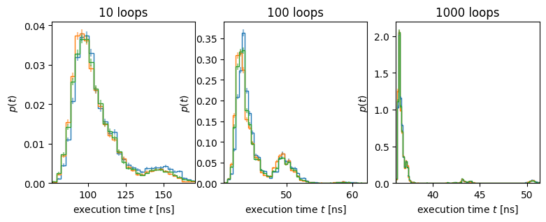
Several things to note here:
The distribution is typically multi-modal, with a large cluster for small times, but several clusters at larger times, presumably when the calculations were interrupted by some other process on the computer.
Small numbers of loops have significant errors: this is because no effort is made to remove systematic timing effects (see [Moreno and Fischmeister, 2017] for some ideas that we may revisit later).
We have included error bars in the histogram assuming that the samples are distributed according to some underlying PDF. Often the model of an underlying CDF is not very good, especially as we increase the number of loops.
These indicate that our idea of interrupts affecting the timing has validity and demonstrates one of the issues with timing: to deal with measurement issues, we typically want enough loops to ensure that the measured time is larger compared with timing uncertainties. However, this increases the likelihood that system interrupts will contaminate the results. It also indicates that the distribution of interrupts is not very random.
A better approach to test this is to look at the empirical CDF (eCDF), where we can use the Kolmogorov-Smirnov to quantify this assumption. For now we will proceed to develop the theory assuming our model of a fixed PDF \(p(t)\) is correct. For definiteness we will the sum of two shifted Wald distribution:
import numpy as np
from scipy.stats import wald

class ExecutionModel:
    modes = (1, 4)
    ratios = (5, 1)
    rng = np.random.default_rng(seed=2)

    def generate(self, size=1):
        rng = self.rng
        p = np.divide(self.ratios, np.sum(self.ratios))
        return (rng.choice(self.modes, size=size, p=p)
            + wald.rvs(size=size, random_state=self.rng))

    def pdf(self, t):
        ps = np.divide(self.ratios, np.sum(self.ratios))
        return sum(p*wald.pdf(t-mode) for mode, p in zip(self.modes, ps))

    def cdf(self, t):
        ps = np.divide(self.ratios, np.sum(self.ratios))
        return sum(p*wald.cdf(t-mode) for mode, p in zip(self.modes, ps))

model = ExecutionModel()

Ns = 10000

ts = model.generate(size=Ns)
t0, t1 = np.percentile(ts, [0, 95])
hist_err(ts, bins=500, density=True);
ts_ = np.linspace(t0, t1)
plt.plot(ts_, model.pdf(ts_))
ax = plt.gca()
ax.set(xlim=(t0, t1),
       xlabel=f"mock execution time $t$",
       ylabel="$p(t)$ (PDF)");
ax = plt.twinx()
ax.plot(np.sort(ts), np.arange(len(ts))/len(ts), '--')
ax.plot(ts_, model.cdf(ts_), '--')
ax.set(ylabel="$P(t)$ (CDF)");
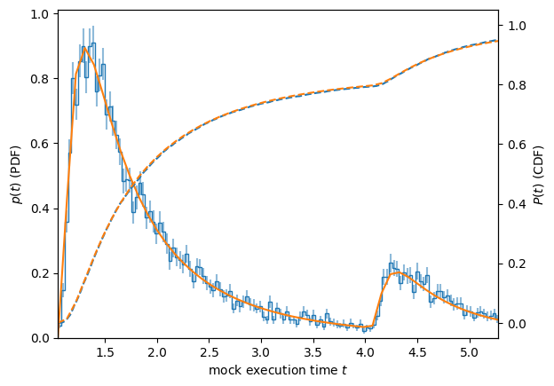
Here we use the notation \(p(t)\) for the PDF and \(P(t)\) for the CDF:
Extremal Value Theory#
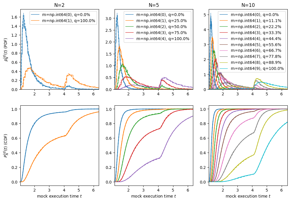
Suppose we measure the execution time \(N=m+n+1\) times. One can show that the percentile
\(q=m/(N-1)\) is distributed as a beta distribution scipy.stats.beta:
Here \(I_{x}(a,b)\) is the regularized incomplete Beta function:
One special case is the distribution of the minimum of \(N\) measurements when \(m=0\):
This is a famous result in extreme value theory. The interpretation is simple: \(1-P(t)\) is the probability of finding a value greater than or equal to \(t\). Thus \(P_{N}^{(0)}(t)\) is simply the probability that all \(N\) values are greater than or equal to \(t\), which is the condition that \(t\) is the minimum value.
Side Problem
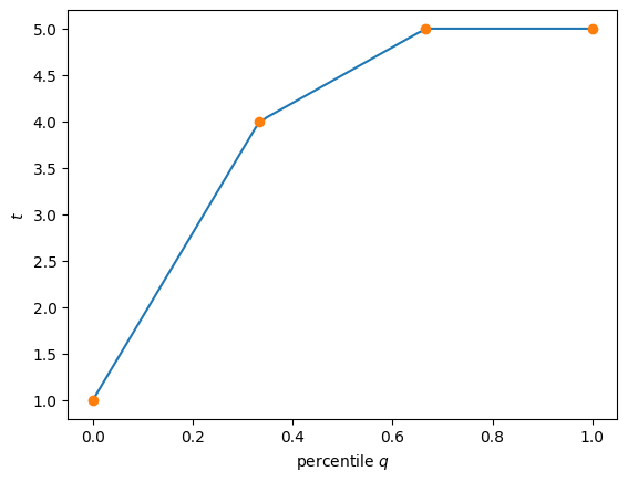
The formulae given here work for percentiles \(q = m/(N-1)\) that lie exactly at the data points. They can be evaluated for fractional \(m\) by using, for example, the gamma function \(m! = \Gamma(m+1)\). What does this imply for how these in-between-percentiles are defined?
Many programs like NumPy define them by linear interpolation. Thus, if the \(q\)’th percentile lies between two data points \(t_a\) and \(t_b\), then the percentile is defined as \(qt_a + (1-q)t_b\) (see below) such that \(t(q)\) is piecewise linear.
Question: what do these formulae imply about how \(t(q)\) is defined for intermediate percentiles \(q \neq m/(N-1)\)?
ts = [1,4,5,5]
q = np.linspace(0, 1)
N = len(ts)
m = np.arange(N)
plt.plot(q, np.percentile(ts, q*100))
plt.plot(m/(N-1), ts, 'o')
ax = plt.gca()
ax.set(xlabel="percentile $q$", ylabel="$t$");
Here we check these formulae by generating some data:
from scipy.special import betainc, factorial

Ns = [1, 2, 3, 4, 5]
Ns = [2, 5, 10]
samples = 10000
scale = 4
fig, axs = plt.subplots(2, len(Ns), figsize=(scale*len(Ns), scale*2))
for i, N in enumerate(Ns):
    ts = model.generate(size=(N, samples))
    t0, t1 = np.percentile(ts.ravel(), [0, 98])
    ms = np.arange(N)
    qs = ms/(N-1)
    percentiles = 100*qs
    Ts = np.asarray(np.percentile(ts, percentiles, axis=0))
    t = np.linspace(t0, t1, 500)
    for j, (m, p) in enumerate(zip(ms, percentiles)):
        label = f"{m=}, q={p:.1f}%"
        ax = axs[0, i]
        plt.sca(ax)
        hist_err(Ts[j], bins=100, density=True, color=f"C{j}", label=label);
        p, P = model.pdf(t), model.cdf(t)
        n = N-m-1
        p_N = factorial(N)/factorial(m)/factorial(n) * P**m * (1-P)**n * p
        ax.plot(t, p_N, f"--C{j}")
        ax.set(xlim=(t0, t1), title=f"{N=}")
        plt.legend()

        ax = axs[1, i]
        plt.sca(ax)
        P_N = betainc(m+1, n+1, P)
        ax.plot(np.sort(Ts[j]), np.arange(samples)/(samples-1), label=label)
        ax.plot(t, P_N, f"--C{j}")
    axs[0, i].set(xlim=(t0, t1))
    axs[1, i].set(xlim=(t0, t1), xlabel=f"mock execution time $t$")
axs[0, 0].set(ylabel="$p_{N}^{(q)}(t)$ (PDF)");
axs[1, 0].set(ylabel="$P_{N}^{(q)}(t)$ (CDF)");
from scipy.special import betainc, factorial

qs = [0, 0.5, 1.0]
Ns = [3, 5, 7, 15]
samples = 10000
scale = 4
fig, axs = plt.subplots(2, len(qs), figsize=(scale*len(qs), scale*2))
data = []
for i, q in enumerate(qs):
    data.append([])
    for j, N in enumerate(Ns):
        ts = model.generate(size=(N, samples))
        m = (N-1)*q
        Ts = np.asarray(np.percentile(ts, 100*q, axis=0))
        data[-1].append(Ts)

data = np.array(data)
for i, q in enumerate(qs):
    t0, t1 = np.percentile(data[i, :].ravel(), [0, 99])
    t = np.linspace(t0, t1, 500)
    for j, N in enumerate(Ns):
        m = (N-1)*q
        n = int(N-m-1)
        Ts = data[i, j]
        label = f"{N=}"
        ax = axs[0, i]
        plt.sca(ax)
        hist_err(Ts, bins=100, density=True, color=f"C{j}", label=label);
        p, P = model.pdf(t), model.cdf(t)
        p_N = factorial(N)/factorial(m)/factorial(n) * P**m * (1-P)**n * p
        ax.plot(t, p_N, f"--C{j}")
        ax.set(xlim=(t0, t1), title=f"$q={q*100:.0f}$%")
        plt.legend()

        ax = axs[1, i]
        plt.sca(ax)
        P_N = betainc(m+1, n+1, P)
        ax.plot(np.sort(Ts), np.arange(samples)/(samples-1), label=label)
        ax.plot(t, P_N, f"--C{j}")
        ax.set(xlim=(t0, t1), xlabel=f"mock execution time $t$")
axs[0, 0].set(ylabel="$p_{N}^{(q)}(t)$ (PDF)");
axs[1, 0].set(ylabel="$P_{N}^{(q)}(t)$ (CDF)");
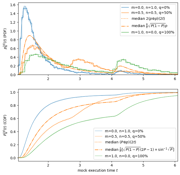
Consider again the side-problem. With \(N=2\) and NumPy’s interpolation formulation, the median will now be the mean, hence the distribution will be the convolution:
NumPy definition of the median as the arithmetic mean of the two values:
\[\begin{gather*} p_{2}^{(50\%)}(t) = 2(p ⊛ p)(2t)\\ P_{2}^{(50\%)}(t) = (P ⊛ p)(2t). \end{gather*}\]Extension of the formulae given here. What combination of gives this?
\[\begin{gather*} p_{2}^{(50\%)}(t) = \frac{8}{\pi}\sqrt{P(t)\bigl(1-P(t)\bigr)}p(t)\\ P_{2}^{(50\%)}(t) = \frac{2}{\pi}\Big(\sqrt{P(1-P)}(2P-1)+\sin^{-1}\sqrt{P}\Bigr). \end{gather*}\]
The question posed above for the median is to find the function \(f_{0.5}(t_1, t_2)\) such that
What about other means? The geometric mean gives
from scipy.special import betainc, factorial

N = 2
samples = 10000
scale = 4
fig, axs = plt.subplots(2, 1, figsize=(scale*2, scale*2))
ts = model.generate(size=(N, samples))
qs = [0, 0.5, 1.0]
Ts = np.asarray([np.percentile(ts, 100*q, axis=0) for q in qs])
t0, t1 = np.percentile(Ts.ravel(), [0, 98])
t = np.linspace(t0, t1, 500)
p, P = model.pdf(t), model.cdf(t)
for i, q in enumerate(qs):
    m = (N-1)*q
    n = N - m - 1
    label = f"{m=:.1f}, {n=:.1f}, q={100*q:.0f}%"
    ax = axs[0]
    plt.sca(ax)
    hist_err(Ts[i], bins=100, density=True, color=f"C{i}", label=label)
    p_N = factorial(N)/factorial(m)/factorial(n) * P**m * (1-P)**n * p
    ax.plot(t, p_N, f"--C{i}", lw=0.7)
    ax.set(xlim=(t0, t1))

    if N == 2 and q == 0.5:
        # Plot convolution:
        t_ = np.linspace(1, 2*t1, 2*len(t))
        p_ = model.pdf(t_)
        p_N_mean = 2*np.convolve(p_, p_, mode='full')[::2] * np.diff(t_).mean()
        ax.plot(t_, p_N_mean, f":C{i}",
                label=r"median $2(p ⊛ p)(2t)$")
        ax.plot(t, 8/np.pi * np.sqrt(P*(1-P))*p, f"-.C{i}",
                label=r"median $\frac{8}{\pi}\sqrt{P(1-P)}p$")

    ax = axs[1]
    plt.sca(ax)
    P_N = betainc(m+1, n+1, P)
    ax.plot(np.sort(Ts[i]), np.arange(samples)/(samples-1), label=label, lw=0.5)
    ax.plot(t, P_N, f"--C{i}", lw=0.7)

    if N == 2 and q == 0.5:
        t_ = np.linspace(1, 2*t1, 2*len(t))
        p_ = model.pdf(t_)
        P_ = model.cdf(t_)
        P_N_mean = np.convolve(P_, p_, mode='full')[::2] * np.diff(t_).mean()
        ax.plot(t_, P_N_mean, f":C{i}",
                label=r"median $(P ⊛ p)(2t)$")
        ax.plot(t, 2/np.pi * (np.sqrt(P*(1-P))*(2*P-1) + np.arcsin(np.sqrt(P))),
                f"-.C{i}",
                label=r"median $\frac{2}{\pi}[\sqrt{P(1-P)}(2P-1) + \sin^{-1}\sqrt{P}]$")

    ax.set(xlim=(t0, t1), xlabel=f"mock execution time $t$")

for ax in axs:
    plt.sca(ax)
    plt.legend();

axs[0].set(ylabel="$p_{N}^{(q)}(t)$ (PDF)");
axs[1].set(ylabel="$P_{N}^{(q)}(t)$ (CDF)");