Model Fitting E.g. 1: Cosine#
Here we go through the step-by-step procedure for fitting data to the following model:
We shall assume that the errors are independently distributed, considering both the case of gaussian errors, and non-gaussian:
We start with the gaussian case, and assume that the errors are sufficiently small that the standard analysis techniques based on \(\chi^2(\vect{a})\) apply as discussed in chapter 15 of [Press et al., 2007]. We then test these using Monte Carlo (MC) and then use an MCMC approach to solve the general case.
To make our examples mode modular, I am going to use a class to represent the mock experiment. We can specify the nature of the errors, and generate sample experiments for our analysis.
from IPython.display import Latex
from collections import namedtuple
from functools import partial
import uncertainties
from uncertainties import unumpy as unp
from scipy.optimize import least_squares
import scipy.stats
sp = scipy


class Experiment:
    """Class representing a mock experiment.

    Attributes
    ----------
    a : Params
        Exact parameter values.
    ts : array-like
        Times at which to sample the function.
    ys : array-like
        Exact values sampled at the specified times.
    ydata : array-like
        Simulated measurement.
    """
    Params = namedtuple("Params", ["w", "c", "A", "phi"])
    labels = [r"$\omega$", r"$c$", r"$A$", r"$\phi$"]

    def __init__(self,
                 random=np.random.default_rng(seed=2).normal,
                 ts=np.linspace(0, 10.0, 7),
                 sigmas=0.5,
                 a=Params(w=2 * np.pi / 5, c=2.1, A=3.4, phi=5.6)):
        """Constructor.

        Arguments
        ---------
        random : function
            Random generator for the errors.  Should return
            sample errors from a normalized distribution.  Will
            be scaled by sigmas to get the actual errors.
        ts : array-like
            Range of times at which to sample the function.
        sigmas : float or array-like
            Errors.
        """
        self.random = random
        self.ts = np.asarray(ts)
        self.a = self.Params(*a)
        self.ys = self.f(self.ts, *self.a)

        # Allow sigmas to be a float
        self.sigmas = np.zeros_like(ts) + sigmas
        self.ydata = self.measure()

    def f(self, ts=None, *a, np=np):
        """Model function."""
        if not a:
            a = self.a
        if ts is None:
            ts = self.ts

        a = self.Params(*a)

        return a.c + a.A * np.cos(a.w * ts + a.phi)

    def measure(self, ys=None, a=None, sigmas=None):
        """Return `ydata` corresponding to a simulated measuement."""
        if ys is None:
            if a is None:
                ys = self.ys
            else:
                ys = self.f(self.ts, *a)
        if sigmas is None:
            sigmas = self.sigmas
        return self.random(loc=ys, scale=sigmas)

    def residuals(self, a, ydata=None, sigmas=None):
        """Return the residuals for least_square.

        May be overloaded to implement robust fitting models.

        Arguments
        ---------
        a : Params
            Parameter estimate.
        """
        if ydata is None:
            ydata = self.ydata
        if sigmas is None:
            sigmas = self.sigmas
        return (ydata - self.f(self.ts, *a))/sigmas

    FitResults = namedtuple("FitResults",
                            ['a', 'C', 'chi2_r', 'nu', 'a_'])

    def fit(self, ydata=None, sigmas=None):
        """Return `FitResults` from least_squares fit.

        Arguments
        ---------
        ydata : array-like, optional
            Experimental data.  Uses `self.ydata` if not provided.

        Returns
        -------
        a : Params
            Parameter estimates.
        C : array
            Covariance matrix.
        chi2_r : float
            Sum of the residuals normalized by `nu`.
        nu : int
            Effectve number of degrees of freedom.
        a_ : Params
            Correlated parameter estimates using
            `uncertainties.correlated_values`.
        """
        if ydata is None:
            ydata = self.ydata
        if sigmas is None:
            sigmas = self.sigmas

        # Using simple numpy functions, we can compute the jacobian
        # with the complex-step method.
        fun = partial(self.residuals, ydata=ydata, sigmas=sigmas)
        res = least_squares(fun=fun, x0=self.a, jac='cs')
        a = self.Params(*res.x)
        C = np.linalg.inv(res.jac.T @ res.jac)
        a_ = self.correlated_values(a, C)
        r = self.residuals(a, ydata=ydata, sigmas=sigmas)
        nu = len(r) - len(a)
        chi2_r = np.sum(abs(r)**2) / nu

        return self.FitResults(a=a, C=C, chi2_r=chi2_r, nu=nu, a_=a_)

    def correlated_values(self, a, C):
        """Return `Params()` as correlated values using
        `uncertainties.correlated_values`
        """
        return self.Params(*uncertainties.correlated_values(a, C))

    def sample_chi2_r(self, Nsamples=2000, a=None):
        """Return samples of the chi2_r obtained by repeated fitting.

        Arguments
        ---------
        a : Params, optional:
            Parameter values.  If not provided, `self.a` will be
            used, otherwise we will assume that the supplied
            parameters are to be used as a proxy model.
        Nsamples : int
            Number of samples.
        """
        if a is None:
            a = self.a
        chi2_rs = [self.fit(ydata=self.measure(a=a)).chi2_r
                   for n in range(Nsamples)]
        return chi2_rs

    def plot(self, a_=None, a_sigmas=[1, 2, 3, 4], ax=None):
        """Display the current experiment.

        Arguments
        ---------
        a_ : Params
            Correlated best fit parameters.  If provided, this fit
            will be shown with the corresponding confidence regions.
        a_sigmas : array-like
            Bands to show.
        """
        if ax is None:
            fig, ax = plt.subplots()

        ts = np.linspace(self.ts.min(), self.ts.max())
        ax.errorbar(self.ts, self.ydata, yerr=self.sigmas,
                    fmt="C0.", ecolor="C1", label="data")
        ax.plot(ts, self.f(ts), "-C2", label="exact")

        if a_ is not None:
            ys_ = self.f(ts, *a_, np=unp)
            fc = "C3"
            alphas = np.linspace(0.5, 0.1, len(a_sigmas))
            for sigma, alpha in zip(a_sigmas, alphas):
                self.plot_band(ts, ys_, sigma=sigma, ax=ax,
                               fc=fc, alpha=alpha,
                               label=fr"${sigma}\sigma$ band")

        ax.set(xlabel="$t$", ylabel="$f(t)$")

        ax.legend()
        return ax

    def plot_band(self, t, y_, sigma=1, ax=None, **kw):
        """Plot a band using correlated errors in y_."""
        if ax is None:
            ax = plt.gca()
        y = unp.nominal_values(y_)
        dy = unp.std_devs(y_)
        ax.fill_between(t, y-dy*sigma, y+dy*sigma, **kw)
        return ax
Linear Gaussian Approximation#
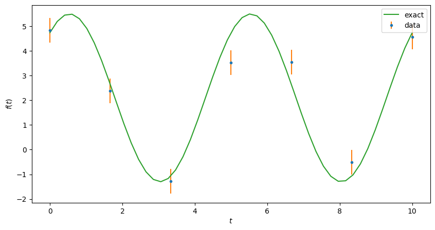
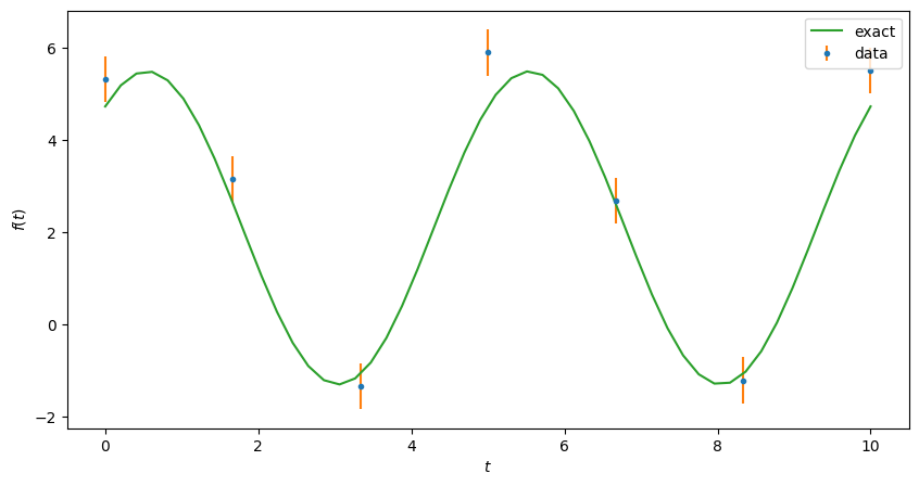
We start with an “exact” solution, then generate some data to analyze at \(N_t\) equally spaced points for \(t \in [0, t_\max]\).
expt = Experiment(ts=np.linspace(0, 10.0, 7),
                  random=np.random.default_rng(seed=2).normal)

fig, ax = plt.subplots(figsize=(10, 5))
expt.plot(ax=ax);
Chi Square Fit#
Now we do the fit. We use scipy.optimize.least_squares() which requires a
function that returns the list of weighted residuals:
This minimizes the following cost function, for which the Hessian is the inverse covariance matrix:
res = expt.fit()

# Since our errors are gaussian and small, we expect that the
# standard chi2 distribution will hold, so we can compute the
# Q values using the corresponding CDF:
Q = 1 - sp.stats.chi2.cdf(res.chi2_r*res.nu, df=res.nu)

Latex(rf"$\chi^2_r = {res.chi2_r:.2g}, \qquad Q = {Q:.2g}$")
Here we have used the Chi-Squared Distribution \(P_{\nu,\chi^2}(\chi^2)\) to calculate the chi-square probability \(Q\), sometimes called the tail distribution:
This is the probability that \(\chi^2\) exceeds the value found, and is the complement of the cumulative distribution function (CDF). This is sometimes called a one-sided \(p\)-value and is used as a test statistic to assess whether or not the model is reasonable. As discussed in section 15.1 of [Press et al., 2007], values of \(Q> 0.001\) are not too bad:
Truly wrong models have values will often be rejected with vastly smaller values of \(Q\), \(10^{-18}\), say.
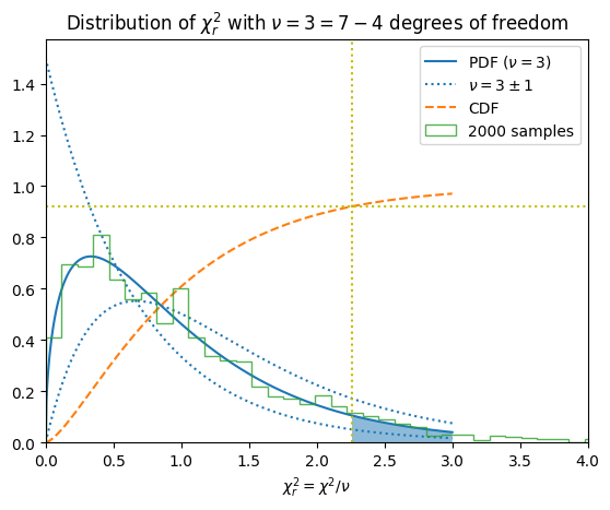
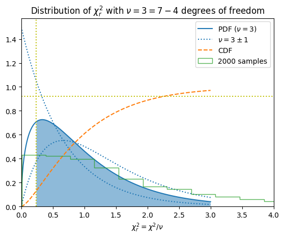
Here we plot the distribution of the reduced chi squared for our dataset with \(\nu = N - M\) degrees of freedom:
Parameter Estimates and Uncertainties#
The results of the fit are characterized by the best-fit parameter values \(\bar{\vect{a}}\) and the covariance matrix \(\mat{C}\) such that, to lowest order, \(\chi^2(\vect{a})\) is quadratic:
The confidence region corresponding to confidence level \(p\) is given by the region within the contour
where the contour \(\chi^2_{p}\) is carefully chosen so that this region contains fraction \(p\) of the samples. This can bed computed from the inverse of the cumulative distribution function (CDF) for the chi squared distribution with \(\nu\) degrees of freedom:
if:
the fit is good,
the posterior distribution is well approximated by a multivariate normal distribution (i.e. if the experimental errors are gaussian and the model is linear in the region of these errors), and
you use the correct value of \(\nu\) corresponding to the number of free parameters you wish to consider. If you want to consider a marginal distribution of \(\tilde{\nu} < \nu\) parameters, then just extract the corresponding \(\tilde{nu}\) rows and columns from \(\mat{C}\) (not \(\mat{C}^{-1}\)).
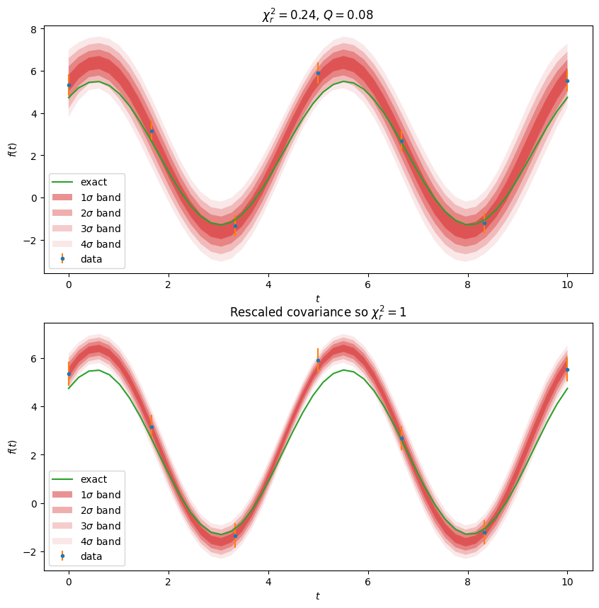
In our case, the errors are gaussian as we saw above, so we can proceed with the simplified approach. What we do here is use the uncertainties package to perform a forward error propagation of the parameter covariance matrix \(\mat{C}\) through to the actual function values for the model \(y = f(x, \vect{a})\). We then treat each \(y\) as a single parameter (\(\tilde{\nu}=1\)) and use the \(n\sigma\) values where \(\sigma\) is the standard deviation computed by the uncertainties package to produce a \(1\sigma\) and \(2\sigma\) uncertainty band corresponding to our parameter values:
a_ = expt.correlated_values(res.a, res.C)
ar_ = expt.correlated_values(res.a, res.C*res.chi2_r)

fig, axs = plt.subplots(2, 1, figsize=(10, 10))
for _a_, ax in zip((a_, ar_), axs):
    expt.plot(a_=_a_, ax=ax)
axs[0].set(title=fr"$\chi^2_r={res.chi2_r:.2f}$, $Q={Q:.2g}$");
axs[1].set(title=r"Rescaled covariance so $\chi^2_r=1$");
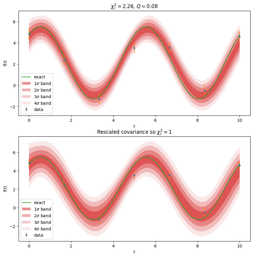
In the lower plot, we have rescaled the covariance matrix \(\mat{C} \rightarrow \chi^2_r \mat{C}\) as if we did not trust our error estimates, and interpreted the large \(\chi^2_r\) value as a sign that we underestimated the errors.
We can now look at some of the marginal distributions. One can use a set of corner plots to summarize this information, but we first do this explicitly.
Single Parameter Distributions#
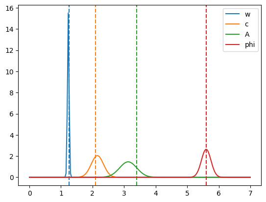
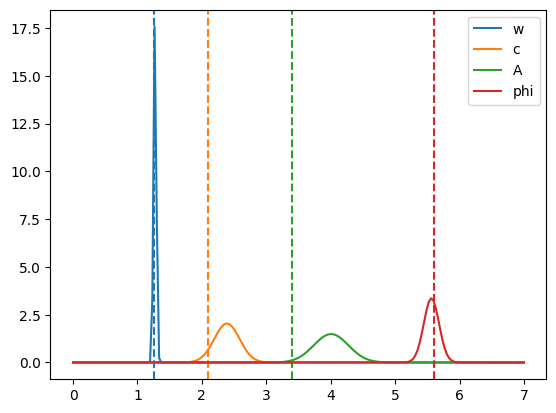
We start with the individual parameter marginal distributions. In this case \(\tilde{\nu} = 1\). Since our posterior is well approximated by a gaussian, we can simply look at the standard deviations given as the square root of the corresponding diagonal entry of the covariance matrix: \(\sigma_i = \sqrt{C_{ii}}\). This is nicely summarized by printing the parameters using the uncertainties package as we show below:
res = expt.fit()
a_, C = res.a_, res.C

fig, ax = plt.subplots()
_x = np.linspace(0, 7, 200)
for _name, _a, _Cii, a in zip(a_._fields, a_, np.diag(C), expt.a):
    print(f"{_name}: {_a:.2uS}, (sqrt(C_ii) = {np.sqrt(_Cii):.2g})")
    l, = ax.plot(_x, sp.stats.norm.pdf(_x, loc=_a.n, scale=_a.s), label=_name)
    ax.axvline([a], ls='--', c=l.get_c())
ax.legend();
w: 1.231(26), (sqrt(C_ii) = 0.026)
c: 2.15(19), (sqrt(C_ii) = 0.19)
A: 3.13(27), (sqrt(C_ii) = 0.27)
phi: 5.60(15), (sqrt(C_ii) = 0.15)
Pairwise Distributions#
Supposed we are most interested in the frequency \(\omega\) and phase \(\phi\). We can consider the marginal distribution of these two parameters by extracting the appropriate columns and rows. Note that we must now choose our contours using \(\tilde{\nu} = 2\). We display these as contours of \(\chi^2\):
res = expt.fit()

a_ = res.a_

i, j = map(a_._fields.index, ['w', 'phi'])
w_, phi_ = a_.w, a_.phi

# Extract rows and colums.  Note: C[[i, j], [i, j]] does not work.
Cij = C[[i, j], :][:, [i, j]]

# We can also do this with the uncertainties package
from uncertainties import covariance_matrix
assert np.allclose(Cij, covariance_matrix([w_, phi_]))

_sigma = 5
ws, phis = np.meshgrid(
  np.linspace(w_.n-_sigma*w_.s, w_.n+_sigma*w_.s, 200),
  np.linspace(phi_.n-_sigma*phi_.s, phi_.n+_sigma*phi_.s, 200))

# Deviation matrix to calculate chi2
dws_phis = np.array([ws-w_.n, phis-phi_.n])

# This is just the matrix product, but we want to do this
# over a bunch of parameter values, so we use einsum.
dchi2 = np.einsum('ij,ixy,jxy->xy',
                   np.linalg.inv(Cij), dws_phis, dws_phis)

# Use a normal distribution to compute the confidence levels
sigmas_ = np.array([1, 2, 3, 4])
ps = sp.stats.norm.cdf(sigmas_) - sp.stats.norm.cdf(-sigmas_)

# Now use chi2 distribution to get the corresponding contours
levels = sp.stats.chi2.ppf(ps, df=2)
fig, ax = plt.subplots(figsize=(10, 6))
_cs = ax.contour(ws, phis, dchi2, levels=levels, cmap="winter")
fmt = dict([(_l, fr"${_n}\sigma$")
            for _l, _n, _p in zip(levels, sigmas_, ps)])

# Draw single-parameter confidence limits to show that
# they are smaller.
for _n, _sigma in enumerate(sigmas_):
    kw = dict(c=_cs.get_edgecolors()[_n],
              alpha=0.5, zorder=-100)
    for _s in [1, -1]:
        ax.axhline(phi_.n + _s*_sigma*phi_.s, ls=":", **kw)
        ax.axvline(w_.n + _s*_sigma*w_.s, ls="--", **kw)
ax.clabel(_cs, _cs.levels, inline=True, fmt=fmt, fontsize=10)
ax.set(xlabel="$\omega$", ylabel="$\phi$");
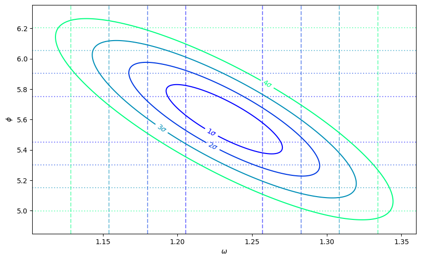
We show the \(1\sigma\), \(2\sigma\), \(3\sigma\), and \(4\sigma\) \(\tilde{\nu} = 2\)-parameter confidence regions demonstrating the correlations between \(\omega\) and \(\phi\). For comparison, we show the corresponding 1-parameter regions as dotted lines. E.g. for the \(1\sigma\) confidence regions, the same amount of posterior probability (68.27%) lies within the center blue ellipse as lies between the central vertical blue dashed lines, or between the central horizontal blue dotted lines.
In other words, the single-parameter confidence regions include points outside of the 2-parameter ellipse, hence must be smaller as shown to keep the same probability.
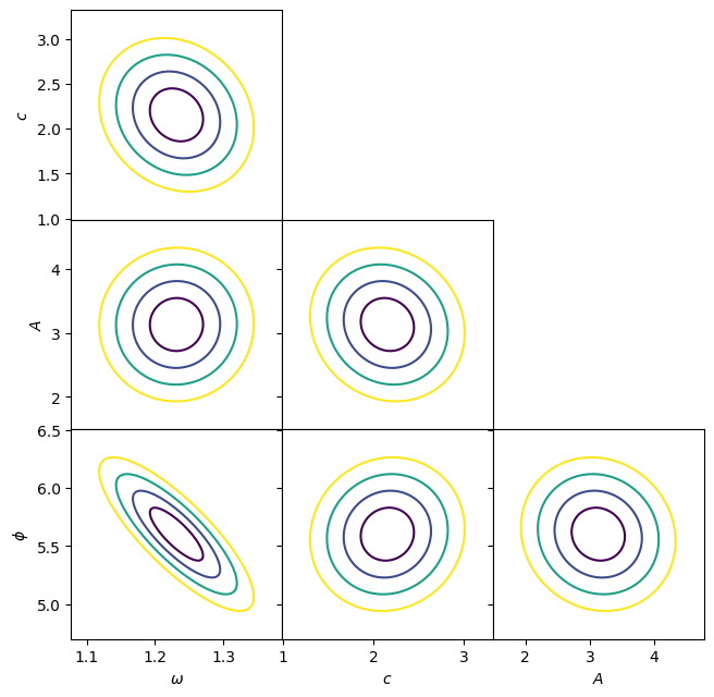
Here is the full corner plot using phys_581.plotting.corner_plot():
from phys_581.plotting import corner_plot
res = expt.fit()

fig, axs = corner_plot(res.a_, labels=expt.labels)
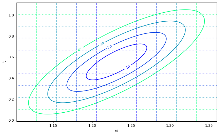
Change of Variables#
To compute a change of variables, we need to keep track of the Jacobian of the transformation so we can properly transform the covariance matrix. The uncertainties package does this automatically, computing the derivatives with automatic differentiation. This is only valid if the errors are small enough that the model is approximately linear, but is very convenient. Here we replace \(\phi\) with the location of the peak \(t_0\):
# make sure t0_ is positive and small by making phi0_ between -2pi and 0
phi0_ = phi_ - phi_.n + phi_.n % (2*np.pi) - 2*np.pi
t0_ = - phi0_ / w_

Cij = covariance_matrix([w_, t0_])

_sigma = 5
ws, t0s = np.meshgrid(
  np.linspace(w_.n-_sigma*w_.s, w_.n+_sigma*w_.s, 200),
  np.linspace(t0_.n-_sigma*t0_.s, t0_.n+_sigma*t0_.s, 200))

# Deviation matrix to calculate chi2
dws_t0s = np.array([ws-w_.n, t0s-t0_.n])
dchi2 = np.einsum('ij,ixy,jxy->xy',
                   np.linalg.inv(Cij), dws_t0s, dws_t0s)

# Now use chi2 distribution to get the corresponding contours
fig, ax = plt.subplots(figsize=(10, 6))
_cs = ax.contour(ws, t0s, dchi2, levels=levels, cmap="winter")
fmt = dict([(_l, fr"${_n}\sigma$")
            for _l, _n, _p in zip(levels, sigmas_, ps)])

# Draw single-parameter confidence limits to show that
# they are smaller.
for _n, _sigma in enumerate(sigmas_):
    kw = dict(c=_cs.get_edgecolors()[_n],
              alpha=0.5, zorder=-100)
    for _s in [1, -1]:
        ax.axhline(t0_.n + _s*_sigma*t0_.s, ls=":", **kw)
        ax.axvline(w_.n + _s*_sigma*w_.s, ls="--", **kw)
ax.clabel(_cs, _cs.levels, inline=True, fmt=fmt, fontsize=10)
ax.set(xlabel="$\omega$", ylabel="$t_0$");
Non-Gaussian Errors#
We now repeat the analysis, but with non-gaussian errors. Instead, we use the Gumbel distribution:
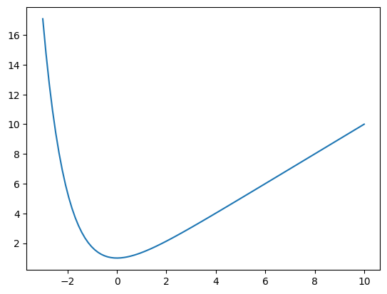
If we consider the normalized errors \(\tilde{e}_n\), they are distributed as:
We can use this to generate the various simulated \(P_{\nu}(\chi^2)\) distributions for Gumbel distributed errors.
en = np.linspace(-3, 10, 100)
plt.plot(en, en + np.exp(-en));
from scipy.interpolate import InterpolatedUnivariateSpline, UnivariateSpline
rng = np.random.default_rng(seed=2)

def get_cdf_ppf(samples=None):
    """Return interpolated cdf and ppf functions.

    Results
    -------
    cdf : function
        Cumulative distribution function `q=cdf(chi2_r)`.
    ppf : function
        Percent point function (inverse of `cdf`).
    """
    Ns = len(samples)
    ps = np.linspace(0, 1, Ns)
    x = sorted(samples)
    cdf = InterpolatedUnivariateSpline(x, ps, k=1, ext='const')
    ppf = InterpolatedUnivariateSpline(ps, x, k=1, ext='const')
    return cdf, ppf

def get_chi2_cdf_ppf(nu=1, random=rng.normal, Ns=10000):
    """Return `(cdf, pdf, samples)` for the chi2 distribution.

    Arguments
    ---------
    nu : int
        Degrees of freedom.
    random : function
        Random number generator for errors.
    Ns : int
        Number of samples.
    """
    en = random(size=(Ns, nu))
    chi2 = (en**2).sum(axis=-1)
    cdf, ppf = get_cdf_ppf(chi2)
    return cdf, ppf, chi2
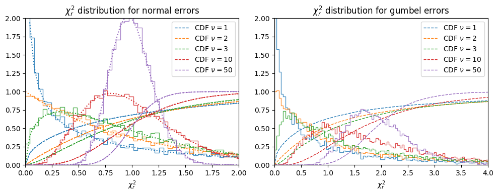
On the left we show the CDF and PDF histogram for \(\chi^2_r\) generated from a sample of random numbers for a standard normal distribution, comparing with the analytic forms (dotted lines). On the right we use the same method to compute the CDF for the standard Gumbel distribution.
We now generate experimental data and proceed with an analysis:
# Randomly generated data...
# An "Experiment" with non-gaussian errors.

expt = Experiment(ts=np.linspace(0, 10.0, 7),
                  random=np.random.default_rng(seed=2).gumbel)

fig, ax = plt.subplots(figsize=(10, 5))
expt.plot(ax=ax);
Chi Square Fit#
Parameter Estimates and Uncertainties#
a_ = expt.correlated_values(res.a, res.C)
ar_ = expt.correlated_values(res.a, res.C*res.chi2_r)

fig, axs = plt.subplots(2, 1, figsize=(10, 10))
for _a_, ax in zip((a_, ar_), axs):
    expt.plot(a_=_a_, ax=ax)
axs[0].set(title=fr"$\chi^2_r={res.chi2_r:.2f}$, $Q={Q:.2g}$");
axs[1].set(title=r"Rescaled covariance so $\chi^2_r=1$");
Single Parameter Distributions#
Unlike the case with gaussian errors, the parameter estimates are no longer consistent with the estimates.
res = expt.fit()
a_, C = res.a_, res.C

fig, ax = plt.subplots()
_x = np.linspace(0, 7, 200)
for _name, _a, _Cii, a in zip(a_._fields, a_, np.diag(C), expt.a):
    print(f"{_name}: {_a:.2uS}, (sqrt(C_ii) = {np.sqrt(_Cii):.2g})")
    l, = ax.plot(_x, sp.stats.norm.pdf(_x, loc=_a.n, scale=_a.s), label=_name)
    ax.axvline([a], ls='--', c=l.get_c())
ax.legend();
w: 1.272(22), (sqrt(C_ii) = 0.022)
c: 2.39(20), (sqrt(C_ii) = 0.2)
A: 4.01(27), (sqrt(C_ii) = 0.27)
phi: 5.56(12), (sqrt(C_ii) = 0.12)
Chi Square Fit#
res = least_squares(fun=partial(get_residuals, ydata=ydata),
                    x0=a_exact, jac='cs')
p = Params(*res.x)
C = np.linalg.inv(res.jac.T @ res.jac)
r = get_residuals(p)
nu = len(r) - len(p)
chi2_r = np.sum(abs(r)**2) / nu
Q_wrong = 1 - sp.stats.chi2.cdf(chi2_r*nu, df=nu)

cdf_gumbel, pdf_gumbel, chi2s_gumbel = get_chi2_cdf_ppf(nu=nu, random=rng.gumbel)
Q = 1 - cdf_gumbel(chi2_r*nu)

Latex(r", \qquad ".join([
    rf"$\chi^2_r = {chi2_r:.2g}",
    rf"Q = {Q:.2g}",
    rf"Q_{{\mathrm{{wrong}}}} = {Q_wrong:.2g}$"]))
---------------------------------------------------------------------------
NameError                                 Traceback (most recent call last)
Cell In[18], line 1
----> 1 res = least_squares(fun=partial(get_residuals, ydata=ydata),
      2                     x0=a_exact, jac='cs')
      3 p = Params(*res.x)
      4 C = np.linalg.inv(res.jac.T @ res.jac)

NameError: name 'get_residuals' is not defined
With the non-gaussian errors, estimating the \(Q\) value with the chi squared distribution gives a very wrong interpretation about the quality of the fit. Instead, we must use the corresponding CDF for our Gumbel-distributed errors. To obtain the confidence region with confidence level \(p\), we must find the value of \(\chi^2_p\) where:
This is just the inverse CDF. We can check our method (slowly) by actually fitting the data repeatedly to generate the distribution of \(\chi^2\):
---------------------------------------------------------------------------
NameError                                 Traceback (most recent call last)
Cell In[19], line 5
      2 from functools import partial
      4 Ns = 2000  # number of samples
----> 5 chi2s_data = np.array([nu*get_chi2_r(random=rng.gumbel) for n in range(Ns)])
      6 chi2s_normal = np.array([nu*get_chi2_r(random=rng.normal) for n in range(Ns)])
      8 cdf_data, ppf_data = get_cdf_ppf(chi2s_data)

NameError: name 'get_chi2_r' is not defined
fig, ax = plt.subplots()
random = rng.gumbel
for Ns in [500, 1000]:
    chi2s_data = np.array([nu*get_chi2_r(random=random) for n in range(Ns)])
    cdf_data, ppf_data = get_cdf_ppf(chi2s_data)
    cdf_gumbel, pdf_gumbel, chi2s_gumbel = get_chi2_cdf_ppf(nu=nu, random=random)
    ax.plot(_chi2_r, cdf_data(nu*_chi2_r), '-', label=f"data {Ns}")
ax.plot(_chi2_r, cdf_gumbel(nu*_chi2_r), ':', label="gumbel")
ax.legend()
---------------------------------------------------------------------------
NameError                                 Traceback (most recent call last)
Cell In[20], line 4
      2 random = rng.gumbel
      3 for Ns in [500, 1000]:
----> 4     chi2s_data = np.array([nu*get_chi2_r(random=random) for n in range(Ns)])
      5     cdf_data, ppf_data = get_cdf_ppf(chi2s_data)
      6     cdf_gumbel, pdf_gumbel, chi2s_gumbel = get_chi2_cdf_ppf(nu=nu, random=random)

NameError: name 'get_chi2_r' is not defined
---------------------------------------------------------------------------
NameError                                 Traceback (most recent call last)
Cell In[21], line 11
      8 ax.plot(_chi2_r, nu*sp.stats.chi2.pdf(nu*_chi2_r, df=nu-1), ":C1", label=rf"$\nu={nu}\pm 1$")
      9 ax.plot(_chi2_r, nu*sp.stats.chi2.pdf(nu*_chi2_r, df=nu+1), ":C1")
---> 11 ax.plot(_chi2_r, cdf_gumbel(nu*_chi2_r), "--C0", label=rf"CDF (Gumbel)")
     12 ax.plot(_chi2_r, sp.stats.chi2.cdf(nu*_chi2_r, df=nu), "--C1", label=rf"CDF $\nu={nu}$")
     14 # Make sure bins end on chi2_r

NameError: name 'cdf_gumbel' is not defined

References#
Samples, samples, everywhere…: A nice overview of different MCMC software accessible with python.