Show code cell content

Hide code cell content

import mmf_setup

mmf_setup.nbinit()
import logging

logging.getLogger("matplotlib").setLevel(logging.CRITICAL)
%matplotlib inline
import numpy as np, matplotlib.pyplot as plt

$\newcommand{\vect}[1]{\mathbf{#1}} \newcommand{\uvect}[1]{\hat{#1}} \newcommand{\abs}[1]{\lvert#1\rvert} \newcommand{\norm}[1]{\lVert#1\rVert} \newcommand{\I}{\mathrm{i}} \newcommand{\ket}[1]{\left|#1\right\rangle} \newcommand{\bra}[1]{\left\langle#1\right|} \newcommand{\braket}[1]{\langle#1\rangle} \newcommand{\Braket}[1]{\left\langle#1\right\rangle} \newcommand{\op}[1]{\mathbf{#1}} \newcommand{\mat}[1]{\mathbf{#1}} \newcommand{\d}{\mathrm{d}} \newcommand{\D}[1]{\mathcal{D}[#1]\;} \newcommand{\pdiff}[3][]{\frac{\partial^{#1} #2}{\partial {#3}^{#1}}} \newcommand{\diff}[3][]{\frac{\d^{#1} #2}{\d {#3}^{#1}}} \newcommand{\ddiff}[3][]{\frac{\delta^{#1} #2}{\delta {#3}^{#1}}} \newcommand{\floor}[1]{\left\lfloor#1\right\rfloor} \newcommand{\ceil}[1]{\left\lceil#1\right\rceil} % The following allows KaTeX to render these for significantly improved % performance on CoCalc. \newcommand{\DeclareMathOperator}[2]{\newcommand{#1}{#2}} \DeclareMathOperator{\Tr}{Tr} \DeclareMathOperator{\erf}{erf} \DeclareMathOperator{\erfi}{erfi} \DeclareMathOperator{\sech}{sech} \DeclareMathOperator{\sn}{sn} \DeclareMathOperator{\cn}{cn} \DeclareMathOperator{\dn}{dn} \DeclareMathOperator{\sgn}{sgn} \DeclareMathOperator{\order}{O} \DeclareMathOperator{\diag}{diag} % \newcommand{\mylabel}[1]{\label{#1}\tag{#1}} \newcommand{\degree}{\circ}$

This cell adds /home/docs/checkouts/readthedocs.org/user_builds/wsu-phys-581-computation/checkouts/latest/src to your path, and contains some definitions for equations and some CSS for styling the notebook. If things look a bit strange, please try the following:

• Choose "Trust Notebook" from the "File" menu.
• Re-execute this cell.
• Reload the notebook.

Gaussian Processes (Theory)

Here we follow chapter 6 of [Rasmussen and Williams, 2006]. The domain of discourse is a reproducing kernel Hilbert space (RKHS). We start with the appropriate definitions:

We will work with complex Hilbert spaces, since these results simplify trivially to real Hilert spaces.

Definition 1 (Hilbert space)

A Hilbert space \(\mathcal{H}\) is a real or complex inner product space that is also a complete metric space with respect to the induced metric.

The relevant space here is that of \(L_2\) functions with the inner product, i.e. over the index space space of \(\mathcal{X} = \mathbb{R}\).

Note: The position of the conjugate on \(a^*\) is the standard in physics, but this convention is often reversed in mathematics (see e.g. Wikipedia). Hence, some of our formula will appear reversed compared to the literature.

\[\begin{gather*} \braket{a, b}_g = \int g(x)\d{x}\; a^*(x)b(x), \qquad \braket{\alpha a, \beta b}_g = \alpha^*\beta\braket{a, b}_g. \end{gather*}\]

We include here the possibility of a “metric” function \(g(x)\) to be discussed later. The notion of completeness means that every Cauchy sequence of points in \(\mathcal{H}\) has a limit also in \(\mathcal{H}\).

Definition 2 (Reproducing kernel Hilbert space (RKHS))

A Hilbert space \(\mathcal{H}\) is called a reproducing kernel Hilbert space (RKHS) if there is a function \(k: \mathcal{X}\times\mathcal{X} \mapsto \mathbb{C}\) called the reproducing kernel which satisfies, for all \(\vect{x} \in \mathcal{X}\):

1. \(k(\vect{x}, \cdot): \mathcal{X}\mapsto \mathbb{C} \in \mathcal{H}\)

2. \(\braket{k(\cdot,\vect{x}), f(\cdot)} = f(\vect{x})\).

In our example space of \(L_2\) functions, the second condition is:

\[\begin{gather*} \int g(y)\d{y}\; k^*(y, x) f(y) = f(x). \end{gather*}\]

As a consequence of the Moore–Aronszajn theorem, the reproducing kernel \(k(\cdot, \cdot)\) is unique in the RKHS, and every symmetric positive definite kernel \(k: \mathcal{X}\times \mathcal{X} \mapsto \mathbb{C}\), there is a unique Hilbert space of functions on \(\mathcal{X}\) for which \(k\) is a reproducing kernel.

To clarify this, consider functions sampled at a discrete set of points \(x_i\) such that \(f_i = f(x_i)\) can be thought of as a finite-dimensional complex vector \(\vect{f}\). To be definite, consider equally spaced points with spacing \(\delta_{x}\) so that the inner-product is:

\[\begin{gather*} \braket{a,b}_{g} = \sum_{i} \overbrace{g(x_i)\delta_{x}}^{G_{ii}}\; a^*(x_i) b(x_i) = \sum_{ij} a^*_i G_{ij} b_j = \vect{a}^\dagger \mat{G} \vect{b}, \end{gather*}\]

where the metric function \(g(x)\) and integration measure have been packaged into the matrix

\[\begin{gather*} \mat{G} = \delta_{x}\begin{pmatrix} g(x_0)\\ & g(x_1)\\ & & \ddots \end{pmatrix} = \begin{pmatrix} G_{00}\\ & G_{11}\\ & & \ddots \end{pmatrix} \end{gather*}\]

Here we sometimes call the matrix \(\mat{G}\) “the metric”, and we can generalize to situations where it is not necessarily diagonal. However, to be a proper inner product space, \(\mat{G}\) must be Hermitian positive definite. We can also represent the kernel \(k(\cdot, \cdot)\) as a matrix:

\[\begin{gather*} [\mat{K}]_{ij} = k(x_i, x_j). \end{gather*}\]

The finite dimensionality removes any subtleties associated with completeness, etc., so we can simply state that a reproducing kernel \(\mat{K}\) satisfies:

\[\begin{gather*} \mat{K}^\dagger \mat{G}\vect{f} = \vect{f}, \qquad \mat{K}^\dagger = \mat{G}^{-1}. \end{gather*}\]

I.e., the kernel \(\mat{K}\) is just the adjoint of the inverse metric. The Moore–Aronszajn theorem is just stating that, for every choice of symmetric positive definite kernel, one obtains a unique inner product space with metric matrix \(\mat{G}\), and vice versa. The symmetric positive definite property ensures that the mapping is one-to-one.

Incomplete

In physics, we usually hide this distinction using bra-ket notation with kets (vectors) \(\ket{a} \in \mathcal{H}\), and defining the bras (forms):

\[\begin{gather*} \bra{a} = \ket{a}... \end{gather*}\]

with vectors \(\ket{f} \in \mathcal{H}\) (using bra-ket notation), and kernels just linear operators \(\op{K}\). Numbers like \(f(\vect{x}) \equiv \braket{x|f}\) are just the coefficients of the vector \(\ket{f}\) in some bass \(\ket{x}\).

I.e., the operator \(\op{K}\) is just the identify on the vector space. This kind of throws out the baby with the bath-water. To see why this is important, consider again

Much of the literature on Gaussian processes uses a slightly different notation with \(\vect{m} \equiv \vect{\mu}\) for the vector of mean values and \(\mat{K} \equiv \mat{\Sigma} \equiv \mat{C}\) for the covariance matrix.

Example Problem: Regression

To make the core ideas here concrete, we consider the problem of trying to learn about a function \(y = f(x)\) where \(f: \mathbb{R}\rightarrow \mathbb{R}\) given some data \(D=\{(x_i, y_i)\} = (\vect{x}, \vect{y})\) distributed as a multivariate Gaussian distribution \(\vect{y} \sim \N(\vect{\mu}, \mat{C})\) with probability distribution function (PDF)

\[\begin{gather*} p_{\N(\vect{\mu}, \mat{C})}(\vect{y}) = \frac{\exp\Bigl(-\tfrac{1}{2}(\vect{y}-\vect{\mu})^\T\mat{C}^{-1}(\vect{y}-\vect{\mu})\Bigr)} {\sqrt{\det\abs{2\pi\mat{C}}}}, \\ [\vect{\mu}]_i = \braket{[\vect{y}]_i}, \qquad [\mat{C}]_{ij} = \kappa(x_i, x_j). \end{gather*}\]

The following provide alternative, but ultimately equivalent, viewpoints of this problem:

1. Linear least-squares fitting. The idea here is to use a set of basis functions \(\phi_n(x)\) and express:

   \[\begin{gather*} f_{\vect{a}}(x) = \sum_{n} a_n \phi_n(x). \end{gather*}\]

   Using Bayes’ theorem, if we have a prior for the parameters \(\vect{a} \sim p(\vect{a})\), then our posterior is:

   \[\begin{gather*} p(\vect{a}|D) \propto \overbrace{\mathcal{L}(\vect{a}|D)}^{p(D|\vect{a})}p(\vect{a}). \end{gather*}\]

   Here the likelihood function \(\mathcal{L}(\vect{a}|D) = p(D|\vect{a})\) is the probability of obtaining the data \(D\) if the true parameter values were \(\vect{a}\). Given our assumption above that \(\vect{y} \sim \N(\vect{\mu}, \mat{C})\), we have:

   \[\begin{gather*} p(D|\vect{a}) = p_{\N(\vect{\mu}, \mat{C})}\Bigl(f_{\vect{a}}(\vect{x})\Bigr). \end{gather*}\]

   If the priors are also distributed as a multivariate Gaussian distribution \(\vect{a} \sim \N(\vect{\mu}_a, \mat{C}_a)\), then we can compute the posterior:

   \[\begin{gather*} p(\vect{a}|D) \propto \overbrace{\mathcal{L}(\vect{a}|D)}^{p(D|\vect{a})}p(\vect{a}). \end{gather*}\]

2. Gaussian Process.

Gaussian Processes

We shall use the notations inspired by [Gelman et al., 2013] and [Melendez et al., 2019].

In simple terms, a Gaussian process is just the generalization of a multivariate Gaussian distribution to infinite-dimensional spaces such as the space of functions. To say that a function \(f: \mathbb{R}\mapsto \mathbb{R}\) is distributed by a Gaussian process

Here the notation \(f \sim \mathcal{P}\) means that \(f\) is distributed according to the probability distribution \(\mathcal{P}\) with probability distribution function (PDF) \(p_{\mathcal{P}}(f)\).

\[\begin{gather*} f \sim \GP[m(x), \kappa(x, x')] \end{gather*}\]

means that, if \(f(x)\) is sampled at any finite set of points \(\vect{x}\) with \(y_i = f(x_i)\), then \(\vect{y}\) is distributed as multivariate Gaussian distribution \(\vect{y} \sim \N(\vect{\mu}, \mat{C})\) with probability distribution function (PDF)

\[\begin{gather*} p_{\N(\vect{\mu}, \mat{C})}(\vect{y}) = \frac{\exp\Bigl(-\tfrac{1}{2}(\vect{y}-\vect{\mu})^\T\mat{C}^{-1}(\vect{y}-\vect{\mu})\Bigr)} {\sqrt{\det\abs{2\pi\mat{C}}}}, \\ [\vect{\mu}]_i = \braket{[\vect{y}]_i}, \qquad [\mat{C}]_{ij} = \kappa(x_i, x_j). \end{gather*}\]

Don’t be scared of infinite dimensional spaces. One can always return to a finite basis \(x_n = x_0 + an\) for \(n\in \{0, 1, \dots, N-1\}\), do ones computations, and then take the continuum \(a \rightarrow 0\) and thermodynamic \(N\rightarrow \infty\) limits. There are cases where these limits do not converge, and these are precisely the subtleties associated with infinite-dimensional spaces, but for most well-behaved (i.e. physical) systems, this poses no difficulty.

I.e. \(\vect{\mu}\) is the vector of mean values and \(\mat{C}\) is the covariance matrix. The functions \(m(x)\) and \(\kappa(x, x')\) are simply the infinite-dimensional 1representations of these in the continuum limit.

Regression

Gaussian processes can be used to perform a generalized linear regression for the function \(y=f(x)\). Consider the aforementioned tabulation \(D=\{(x_i, y_i)\}\) to be “data” from some experiment with correlated Gaussian errors \(\vect{y} \sim \N(\vect{\mu}, \mat{C})\). We can use Bayes’ theorem to update some prior distribution \(f\sim p(f)\):

\[\begin{gather*} p(f|D) \propto \mathcal{L}(f|D)p(f), \qquad \mathcal{L}(f|D) = p(D|f) = p_{\N(\vect{\mu}, \mat{C})}\bigl(f(\vect{x})\bigr). \end{gather*}\]

If the prior is Gaussian process \(f \sim \GP[m(x), \kappa(x, x')]\), then we can compute the posterior analytically.

Details

To see how this works, consider a function \(y_n = f(x_n)\) tabulated at a set of \(N\) points \(x_{n \in \{0, 1, \dots N-1\}}\) with a Gaussian prior \(\vect{y} \sim \N(\vect{\mu}, \mat{C})\). Now consider data \(D\) consisting of a few points \(x_{i \in \{0, 1, M-1\}}\) with experimental errors \(\vect{y}_D \sim \N(\vect{\mu}_D, \mat{C}_D)\). Note, we have not specified which points are where, so we have organized the abscissa so that the experimental data are the first \(M\) points, which need not be adjacent.

We can now express \(\mat{C}\) is block diagonal form with the first block corresponding to the indices where we have data:

\[\begin{gather*} \mat{C} = \begin{pmatrix} \mat{C}_{00} & \mat{C}_{01}\\ \mat{C}_{10} & \mat{C}_{11}. \end{pmatrix} \end{gather*}\]

Organize the points so that the first Consider

Background

Properties of Gaussian Distributions

Here is a quick summary of the relevant properties of multivariate Gaussian distributions. See also Random Variables for additional details.

PDF

The probability distribution function (PDF) for a vector \(\vect{y} \sim \N(\vect{\mu}, \mat{C})\) of variables \(\{y_i\}\) distributed as a multivariate Gaussian distribution (or multivariate normal distribution) is:

\[\begin{gather*} p_{\N(\vect{\mu}, \mat{C})}(\vect{y}) = \frac{\exp\Bigl(-\tfrac{1}{2}(\vect{y}-\vect{\mu})^\T\mat{C}^{-1}(\vect{y}-\vect{\mu})\Bigr)} {\sqrt{\det\abs{2\pi\mat{C}}}}. \end{gather*}\]

Here \(\vect{\mu}\) is the vector of mean values, and \(\mat{C}\) is the covariance matrix.

Product of PDFs

If the covariance matrices are not symmetric, then they must be symmetrized when used in the last relationship:

\[\begin{gather*} (\mat{C}_{c}^{-1} + \mat{C}_{c}^{-1\dagger})\vect{\mu}_c =\\ = (\mat{C}_{a}^{-1} + \mat{C}_{a}^{-1\dagger})\vect{\mu}_a +\\ + (\mat{C}_{b}^{-1} + \mat{C}_{b}^{-1\dagger})\vect{\mu}_b. \end{gather*}\]

The product of the PDFs of multivariate Gaussian distributions with symmetric covariances \(\mat{C} = \mat{C}^\dagger\) is a multivariate Gaussian distribution (but not normalized):

\[\begin{align*} p_{\N(\vect{\mu}_c, \mat{C}_c)}(\vect{y}) & \propto p_{\N(\vect{\mu}_a, \mat{C}_a)}(\vect{y})p_{\N(\vect{\mu}_b, \mat{C}_b)}(\vect{y}), \\ \mat{C}_{c}^{-1} &= \mat{C}_{a}^{-1} + \mat{C}_{b}^{-1}, \\ \mat{C}_{c}^{-1}\vect{\mu}_c &= \mat{C}_{a}^{-1}\vect{\mu}_a + \mat{C}_{b}^{-1}\vect{\mu}_b. \end{align*}\]

I.e. the sums of the inverse covariance matrices add.

Show code cell content

Hide code cell content

from scipy.linalg import expm

rng = np.random.default_rng(seed=1)
N, M = 5, 3
Sinva, Sinvb = rng.random((2, N, N)) - 0.5
#Sinva += Sinva.T
#Sinvb += Sinvb.T
ma, mb = rng.random((2, N, 1)) - 0.5
ys = rng.random((N, M)) - 0.5
Sinvc = Sinva + Sinvb
mc = np.linalg.solve(Sinvc,  Sinva @ ma + Sinvb @ mb)
mc = np.linalg.solve(Sinvc + Sinvc.T,  (Sinva + Sinva.T) @ ma + (Sinvb + Sinvb.T) @ mb)
_c = np.diag(np.exp(-0.5*(ys-mc).T @ Sinvc @ (ys-mc)))
_ab = np.diag(np.exp(-0.5*(ys-ma).T @ Sinva @ (ys-ma) - 0.5*(ys-mb).T @ Sinvb @ (ys-mb)))
_c = _c * _ab[0] / _c[0]
assert np.allclose(_ab, _c)

Marginal Distribution

Recall that the marginal distribution is obtained by integrating over the other variables:

\[\begin{gather*} p(\vect{y}_a) \propto \int \d^{N_b}\vect{y}_b\; p(\vect{y}). \end{gather*}\]

This must be renormalized.

Partition a multivariate Gaussian distribution \(\vect{y} \sim \N_{\vect{y}}(\vect{\mu},\mat{C})\) as

\[\begin{align*} \vect{y} &= \begin{pmatrix} \vect{y}_a\\ \vect{y}_b\\ \end{pmatrix}, & \vect{\mu} &= \begin{pmatrix} \vect{\mu}_a\\ \vect{\mu}_b \end{pmatrix}, & \mat{C} &= \begin{pmatrix} \mat{C}_a & \mat{C}_{ab}\\ \mat{C}_{ba} & \mat{C}_b \end{pmatrix}, \end{align*}\]

where \(\mat{C}_{ba} = \mat{C}_{ab}^\dagger\) for standard distributions \(\mat{C} = \mat{C}^{\dagger}\). The marginal distributions for each partition (integrating over the other variables) are:

\[\begin{align*} \vect{y}_a &\sim \N_{\vect{y}_a}(\vect{\mu}_a, \mat{C}_{a}), \\ \vect{y}_b &\sim \N_{\vect{y}_b}(\vect{\mu}_b, \mat{C}_{b}). \end{align*}\]

I.e. the conditional covariance matrices are just the corresponding sub-blocks of the full covariance matrix.

Conditional Distributions

Partition a multivariate Gaussian distribution \(\vect{y} \sim \N_{\vect{y}}(\vect{\mu},\mat{C})\) as

\[\begin{gather*} \mat{C}^{-1} = \begin{pmatrix} (\mat{C} / \mat{C}_{a})^{-1} & -(\mat{C}/\mat{C}_{b})^{-1}\mat{C}_{ab}\mat{C}_{b}^{-1}\\ -(\mat{C}/\mat{C}_{a})^{-1}\mat{C}_{ba}\mat{C}_{a}^{-1} & (\mat{C} / \mat{C}_{b})^{-1} \end{pmatrix}. \end{gather*}\]

These equations can be easily remembered by considering \(a\) and \(b\) to have different dimensions, and then looking at the indices and noting that adjacent indices much match.

where we have partitioned the inverse covariance here \(\mat{C}^{-1}\) using the Schur complements \(\mat{C} / \mat{C}_{a}\) and \(\mat{C} / \mat{C}_{b}\) of the block matrix \(\mat{C}\):

\[\begin{align*} \mat{C} / \mat{C}_{a} &\equiv \mat{C}_{b} - \mat{C}_{ba}\mat{C}_{a}^{-1}\mat{C}_{ab}, \\ \mat{C} / \mat{C}_{b} &\equiv \mat{C}_{a} - \mat{C}_{ab}\mat{C}_{b}^{-1}\mat{C}_{ba}. \end{align*}. :::{margin} Recall that the conditional distribution is obtained by fixing other variables: \begin{gather*} p(\vect{y}_a|\vect{y}_b) \propto p(\vect{y}). \end{gather*} This must be renormalized. ::: The conditional distributions (holding the other variables fixed) are: \begin{align*} \vect{y}_a &\sim \N_{\vect{y}_a}\Bigl( \vect{\mu}_a + \mat{C}_{ab}\mat{C}_b^{-1}(\vect{y}_b - \vect{\mu}_b),\; \mat{C} / \mat{C}_{a}\Bigr), \\ \vect{y}_b &\sim \N_{\vect{y}_b}\Bigl( \vect{\mu}_b + \mat{C}_{ba}\mat{C}_{a}^{-1}(\vect{y}_a - \vect{\mu}_a),\; \mat{C} / \mat{C}_{b}\Bigr). \end{align*}\]

I.e. the conditional inverse covariance matrices are just the corresponding sub-blocks of the full inverse covariance matrix.

Linear Combinations

If \(\vect{x} \sim \N(\vect{\mu}_x, \mat{C}_x)\) and \(\vect{y} \sim \N(\vect{\mu}_y, \mat{C}_y)\) are independent, then \(\vect{z} = \mat{X}\vect{x} + \mat{Y}\vect{y}\) is distributed as:

\[\begin{gather*} \vect{z} = \mat{X}\vect{x} + \mat{Y}\vect{y} \sim \N\Bigl( \mat{X}\vect{\mu}_x + \mat{Y}\vect{\mu}_y,\; \mat{X}\mat{C}_x\mat{X}^\dagger + \mat{Y}\mat{C}_y\mat{Y}^\dagger \Bigr). \end{gather*}\]

Principle Components, Bases, and Metrics

Consider a multivariate Gaussian distribution normal distribution \(\vect{y} \sim \N(\vect{\mu}, \mat{C})\). If we diagonalize the covariance matrix \(\mat{C} = \mat{U}\mat{D}\mat{U}^{\dagger}\):

\[\begin{gather*} \mat{C} = \overbrace{ \begin{pmatrix} \uvect{u}_0 & \uvect{u}_1 & \cdots \end{pmatrix} }^{\mat{U}} \overbrace{ \begin{pmatrix} \sigma_0^2 \\ & \sigma_1^2\\ & & \ddots \end{pmatrix}}^{\mat{D}} \overbrace{ \begin{pmatrix} \uvect{u}_0^\dagger \\ \uvect{u}_1^\dagger \\ \vdots \end{pmatrix}}^{\mat{U}^\dagger} = \begin{pmatrix} \smash{\overbrace{\uvect{u}_0\sigma_0}^{\vect{u}_0}} & \smash{\overbrace{\uvect{u}_1\sigma_1}^{\vect{u}_1}} & \cdots \end{pmatrix} \begin{pmatrix} \vect{u}_0^\dagger \\ \vect{u}_1^\dagger \\ \vdots \end{pmatrix} \end{gather*}\]

then the columns of \(\mat{U} = [\uvect{u}_0 \; \uvect{u}_1\; \cdots]\) form an orthonormal basis that we can rescale into a set of orthogonal vectors \(\vect{u}_n = \sigma_n\uvect{u}_{n}\) such that

\[\begin{gather*} \vect{y} = \vect{\mu} + \sum_{n} \xi_n\vect{u}_n, \qquad \xi_n \sim \N(0, 1) \end{gather*}\]

where \(\xi_n\) are independent random variables with a standard normal distribution (zero mean and unit covariance). The vectors \(\vect{u}_n\) or the pairs \((\uvect{u}_{n}, \sigma_n)\) are called the principle components. Note that this also follows from the property above of linear combinations of random variables (expressed as a sum of dyads):

\[\begin{gather*} \mat{C} = \sum_{n}\vect{u}_n\vect{u}_n^\dagger. \end{gather*}\]

A somewhat surprising result is that, if we relax the requirement that the vectors \(\vect{u}_n\) be orthogonal, then there are many similar decompositions of \(\vect{y}\) as a linear combination of independent standard normal variables:

\[\begin{gather*} \mat{C} = \sum_{n}\vect{a}_n\vect{a}_n^\dagger = \mat{A}\mat{A}^\dagger, \qquad \mat{A} = \begin{pmatrix} \vect{a}_0 & \vect{a}_1 & \cdots \end{pmatrix}, \end{gather*}\]

where the vectors \(\vect{a}_n\) are linearly independent, but need not be orthogonal.

To see this, construct the singular value decomposition (SVD) for \(\mat{A}\):

\[\begin{gather*} \mat{A} = \mat{U}\sqrt{\mat{D}}\mat{V}^\dagger, \qquad \mat{C} = \mat{A}\mat{A}^\dagger = \mat{U}\mat{D}\mat{U}^\dagger. \end{gather*}\]

If we are careful and arrange the singular values appropriately, then \(\mat{U}\) and \(\mat{D}\) here are the same as in the diagonalization of \(\mat{C}\), but the unitary matrix \(\mat{V}\) is arbitrary. Here we demonstrate numerically in 2D:

Show code cell source

Hide code cell source

def get_V(theta):
    return np.array([[np.cos(theta), -np.sin(theta)], 
                     [np.sin(theta), np.cos(theta)]])

theta0 = np.pi/10
U = get_V(theta=theta0)
D = np.diag([4, 1])
C = U @ D @ U.T
x, y = np.mgrid[-2:2:0.01,-2:2:0.01]
p = np.exp(-np.einsum(
     "axy,bxy,ab->xy", [x, y], [x, y], np.linalg.inv(C))/2)

fig, axs = plt.subplots(1, 2, figsize=(10,5))
ax = axs[0]
ax.contour(x, y, p)
ax.set(aspect=1, xlabel="x", ylabel="y")
_kw = dict(alpha=0.8, width=0.05)
ax.arrow(0, 0, U[0,0], U[1,0], color='k', **_kw)
ax.arrow(0, 0, U[0,1], U[1,1], color='k', **_kw)

angles = []
thetas = np.linspace(0, 2*np.pi, 50)
for theta in thetas:
    A = U @ np.sqrt(D) @ get_V(-theta).T
    a0, a1 = A.T
    norm = np.linalg.norm
    angles.append(180 / np.pi * np.arccos(a0 @ a1 / norm(a0) / norm(a1)))
    assert np.allclose(A @ A.T, C)

for theta, c in [(0.1, 'r'), (0.9, 'g'), (2.4, 'b')]:
    A = U @ np.sqrt(D) @ get_V(-theta).T
    a0, a1 = A.T
    norm = np.linalg.norm
    axs[0].arrow(0, 0, A[0,0], A[1,0], color=c, **_kw)
    axs[0].arrow(0, 0, A[0,1], A[1,1], color=c, **_kw)
    angle = 180 / np.pi * np.arccos(a0 @ a1 / norm(a0) / norm(a1))
    axs[1].plot([theta], [angle], 'o', c=c)

ax = axs[1]
ax.plot(thetas, angles)
ax.set(xlabel=r"$\theta$", ylabel="Angle between $a_0$ and $a_1$");

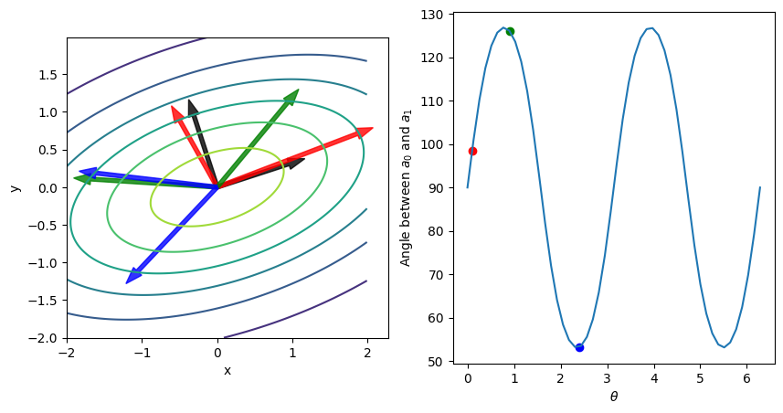
This figure shows contours from a bivariate normal distribution with orthogonal principle components \(\vect{u}_0\) and \(\vect{u}_1\) shown as black vectors. Several equivalent independent but non-orthogonal basis vectors \(\vect{a}_0\) and \(\vect{a}_1\) are shown in different colors. These are generated by a one-dimensional parameterization of the unitary matrix \(\mat{V}(\theta)\). In this case, we can choose any direction \(\uvect{a}_0\), but must construct \(\vect{a}_1\) carefully.

References

• [Gelman et al., 2013]: A good comprehensive reference. Available for non-commercial from the author’s webpage.

• [Melendez et al., 2019]: An application to nuclear theory with associated code gsum.

• [Rasmussen and Williams, 2006]: Another nice book that formed the basis for the implementations in scikit-learn.