Globally Convergent Newton’s Method¶

For finding solutions to non-linear equations \(f(x) = 0\), Newton’s method can converge extremely quickly, roughly doubling the number of digits each step.

\[\begin{gather*} x \mapsto x - \frac{f(x)}{f'(x)}. \end{gather*}\]

However, if the initial state is poorly chosen, it can converge very slowly, or even diverge. By carefully choosing both the form of \(f(x) = 0\) and the initial guess, one can often design an algorithm that will converge for all initial states with a few iterations at most. This is an art rather than a science. Here we show some examples.

Polynomial Inversion¶

An example came up in Random Variables when trying to invert the cumulative distribution function \(C_Z(z) = (-x^3 + 3x + 2)/4\) corresponding to the Thomas-Fermi PDF \(P_Z(z) = 3(1-z^2)/4\). The roots of a polynomial can be found quite efficiently with numpy.roots(), but this returns all 3 roots, and in this case, we want a specific one.

First we plot the function, and note that it is very well approximated by:

\[\begin{gather*} C_Z(z) = \frac{-z^3 + 3z + 2}{4} \approx \frac{1+\sin(\pi z/2)}{2}: \end{gather*}\]

z = np.linspace(-1, 1)
P = np.array([-1, 0, 3, 2])/4

fig, ax = plt.subplots()
ax.plot(z, np.polyval(P, z), label=r"$C_Z(z)$")
ax.plot(z, (1+np.sin(np.pi*z/2))/2, ":", label=r"$[1+\sin(\pi z/2)]/2$")
ax.legend()
ax.set(xlabel="$z$", ylabel="$C_Z(z)$");

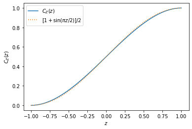
../_images/GloballyConvergentNewton_2_0.png

This suggests a globally convergent strategy for solving \(x = C_Z(z)\):

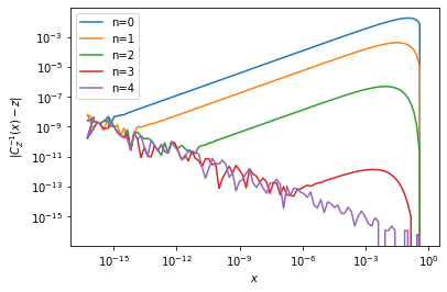
\[\begin{gather*} z_0 = \frac{2}{\pi}\sin^{-1}(2x - 1), \qquad z \mapsto z - \frac{C_Z(z) - x}{C_Z'(x)}. \end{gather*}\]

To check this, we see how many iterations it takes to reach a specified tolerance, and then plot this over the range of inputs:

P = np.array([-1, 0, 3, 2])/4
dP = np.polyder(P)

def C_Z(z):
    return np.polyval(P, z)
    
def C_Z_inv(x, n):
    """Perform `n` steps of Newton's method to invert `x=C_Z(z)`"""
    z = 2/np.pi * np.arcsin(2*x-1)
    for _n in range(n):
        z -= (np.polyval(P, z) - x) / np.polyval(dP, z)
    return z

# Skip endpoints where denominator will be zero
z = np.linspace(-1, 1, 1000)[1:-1]
x = C_Z(z)

fig, ax = plt.subplots()
for n in [0, 1, 2, 3, 4]:
    ax.semilogy(x, abs(C_Z_inv(x, n=n) - z), label=f"n={n}")
ax.legend()
ax.set(xlabel="$x$", ylabel="$|C_Z^{-1}(x)-z|$");

../_images/GloballyConvergentNewton_4_0.png

This shows that we achieve machine precision with 3 iterations if \(x \in [0.2, 0.8]\) and in 4 iterations everywhere else, except near the boundaries. Let’s look a little more closely there (noting that the behavior is symmetric):

# Skip endpoints where denominator will be zero
z = -1 + 10**(np.linspace(-8, 0, 100))
x = C_Z(z)

fig, ax = plt.subplots()
for n in [0, 1, 2, 3, 4]:
    ax.loglog(x, abs(C_Z_inv(x, n=n) - z), label=f"n={n}")
ax.legend()
ax.set(xlabel="$x$", ylabel="$|C_Z^{-1}(x)-z|$");

../_images/GloballyConvergentNewton_6_0.png

The fluctuations here seem to indicate that the issue at the boundary is actually due to roundoff error, so we have are finished with the following:

def C_Z(z, P=[-1, 0, 3, 2]):
    return np.polyval(P, z)/4

def C_Z_inv(x, P=[-1, 0, 3, 2], dP=[-3, 0, 3]):
    """Invert `x=C_Z(z)`"""
    z = 2/np.pi * np.arcsin(2*x-1)
    for _n in range(4):
        z -= (np.polyval(P, z) - 4*x) / (np.polyval(dP, z) + 1e-32)
    return z

x = np.linspace(0, 1, 1000)
z = C_Z_inv(x)
assert np.allclose(C_Z(z), x, atol=1e-15)

Physics 581: Physics Inspired Computational Techniques

Globally Convergent Newton’s Method

Contents

Globally Convergent Newton’s Method¶

Polynomial Inversion¶