Assignment 4: Chaos and Lyapunov Exponents
import mmf_setup;mmf_setup.nbinit()
import logging;logging.getLogger('matplotlib').setLevel(logging.CRITICAL)
%matplotlib inline
import numpy as np, matplotlib.pyplot as plt
This cell adds /home/docs/checkouts/readthedocs.org/user_builds/wsu-phys-581-computation/checkouts/fall-2021 to your path, and contains some definitions for equations and some CSS for styling the notebook. If things look a bit strange, please try the following:
- Choose "Trust Notebook" from the "File" menu.
- Re-execute this cell.
- Reload the notebook.
Assignment 4: Chaos and Lyapunov Exponents
Here we use the ODE solvers to compute the maximum Lyapunov exponent for a system.
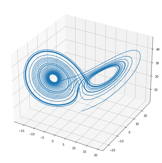
To walk through the code, we look at the Lorenz System, one of the first demonstrations of chaos. This is a set of three coupled non-linear ODEs modeling weather patterns. (For a detailed derivation, see [Fetter and Walecka, 2006].) The system is
This system is chaotic near \(\sigma = 10\), \(\beta = 8/3\), and \(\rho = 28\).
from phys_581_2021.assignment_4 import compute_lyapunov
from scipy.integrate import solve_ivp

sigma = 10.0
beta = 8.0/3
rho = 28.0

q0 = (1.0, 1.0, 1.0)
t0 = 0.0

def compute_dy_dt(t, q):
    """Lorenz equations."""
    x, y, z = q
    return (sigma * (y-x),
            x * (rho - z) - y,
            x * y - beta * z)

# Exploratory run
T = 30.0
res = solve_ivp(compute_dy_dt, y0=q0, t_span=(t0, t0+T), rtol=1e-12, atol=1e-12)
ts = res.t
xs, ys, zs = res.y
fig = plt.figure(figsize=(10,10))
ax = fig.add_subplot(projection='3d')
xs, ys, zs = res.y
ax.plot(xs, ys, zs)
[<mpl_toolkits.mplot3d.art3d.Line3D at 0x7f9bfa17a190>]
fig, ax = plt.subplots(figsize=(10,5))
ax.plot(ts, xs, label='x')
ax.plot(ts, ys, label='y')
ax.plot(ts, zs, label='z')
ax.set(xlabel='t', ylabel='x, y, z')
ax.legend()
<matplotlib.legend.Legend at 0x7f9bfa348340>
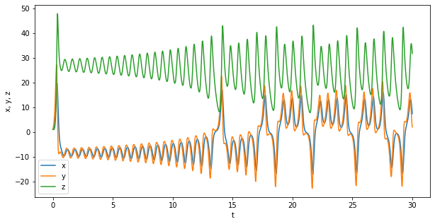
Looking at these plots, we see that it seems to have taken the initial state about \(T=15\) to get close to the attractor where the generic behaviour begins. After this, we see that orbits have a period of about \(T \approx 1\) while it takes about \(T \approx 5\) for the particle to switch between lobes. We expect the chaotic behaviour to be associated with the later phenomenon, so we choose our dt=10.
Nsamples = 200
min_norm = 1e-7
q0 = (1.0, 1.0, 1.0)
t0 = 0.0
dt = 10.0
lams, ts, ys, dys = compute_lyapunov(
    compute_dy_dt,
    y0=q0,
    t0=t0,
    min_norm=min_norm,
    dt=dt,
    Nsamples=Nsamples,
    debug=True)

# Here is the mean and the standard error of the mean
print(np.mean(lams), np.std(lams)/np.sqrt(len(lams)))
0.8664846382859411 0.010858252871237034
fig, ax = plt.subplots(figsize=(10, 5))
for n, t_ in enumerate(ts):
    ls, lw = '-', 0.2
    label = None
    if n < 3:
        ls = '-'
        lw = 1.2
        label = f"n={n}"
    ax.semilogy(t_-t_[0], np.linalg.norm(dys[n], axis=0),
                lw=lw, ls=ls, label=label)

dts = np.linspace(0, 10)
lam0, dlam0 = np.mean(lams), np.std(lams)
ax.fill_between(dts,
                min_norm*np.exp((lam0-dlam0)*dts),
                min_norm*np.exp((lam0+dlam0)*dts), alpha=0.3)
ax.fill_between(dts,
                min_norm*np.exp((lam0-2*dlam0)*dts),
                min_norm*np.exp((lam0+2*dlam0)*dts), alpha=0.2)
ax.set(xlabel="dt", ylabel='norm(dy)', xlim=(0, dt))
ax.legend();
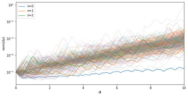
Here we plot the norm of the deviations as a function of the time evolution for 100 samples. We plot a 3 of the first trajectories demonstrating that the first few do not demonstrate typical behavior. There are two potential reason for this:
The initial point did not lie on the attractor, so it takes some time to approach. From the first investigation, we found this took between \(T=10\) and \(T=20\) – the first couple of samples here.
The initial
dymight not point in the direction of the maximal Lyapunov eigenvector. We expect the separation between the two largest exponents to grow as \(e^{(\lambda_0 - \lambda_1)t}\). As you should find, the maximal Lyapunov exponent for these parameter values is about \(\lambda_0 = 0.86\). One can find that, for the Lorenz system with these parameters, the next exponent is negative. Thus, the eigenvector corresponding to the maximal exponent \(\lambda_0\) will dominate in a time \(T \gtrapprox \ln(10^{7})/0.86 \approx 18\).
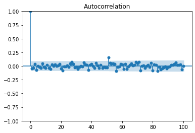
These timescales are consistent with the observation that generic behavior is seen after the first three samples. We further confirm this by plotting the autocorrelation function:
from statsmodels.graphics.tsaplots import plot_acf
plot_acf(lams[:], lags=100);
[I 07:39:37 numexpr.utils] NumExpr defaulting to 2 threads.
/home/docs/checkouts/readthedocs.org/user_builds/wsu-phys-581-computation/conda/fall-2021/lib/python3.9/site-packages/statsmodels/compat/pandas.py:61: FutureWarning: pandas.Int64Index is deprecated and will be removed from pandas in a future version. Use pandas.Index with the appropriate dtype instead.
  from pandas import Int64Index as NumericIndex
/home/docs/checkouts/readthedocs.org/user_builds/wsu-phys-581-computation/conda/fall-2021/lib/python3.9/site-packages/scipy/stats/_ksstats.py:74: RuntimeWarning: invalid value encountered in ldexp
  _EP128 = np.ldexp(np.longdouble(1), _E128)
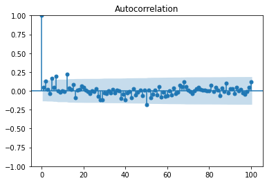
(See Autocorrelation of Time Series Data in Python for a discussion about how to interpret this plot.)
To deal with this manually, we first evolve the initial state a bit. Then we generate some samples to analyze statistically.
min_norm = 1e-7

# First evolve four times to relax
lams, ts, ys, dys = compute_lyapunov(
    compute_dy_dt,
    y0=q0,
    t0=t0,
    min_norm=min_norm,
    dt=10.0,
    Nsamples=4,
    debug=True)
y0 = ys[-1][:, -1]
dy0 = dys[-1][:, -1]

# Now get the data
lams, ts, ys, dys = compute_lyapunov(
    compute_dy_dt,
    y0=y0,
    dy0=dy0,
    t0=t0,
    min_norm=min_norm,
    dt=10.0,
    Nsamples=500,
    debug=True)
lams = np.asarray(lams)
import scipy.stats
from uncertainties import ufloat
sp = scipy
def analyze(lams):
    _lams = np.array(sorted(lams))
    dist = sp.stats.norm(loc=_lams.mean(), scale=_lams.std())
    kernel = sp.stats.gaussian_kde(_lams)

    fig, ax = plt.subplots()
    ax.hist(lams, bins=50, density=True, alpha=0.5)
    ax.plot(_lams, dist.pdf(_lams), '-', label='Gaussian')
    ax.plot(_lams, kernel.pdf(_lams), '--', label='kde')
    lam0 = ufloat(_lams.mean(), _lams.std()/np.sqrt(len(_lams)))
    ax.axvspan(lam0.n - 2*lam0.s, lam0.n + 2*lam0.s, fc='y', alpha=1)
    ax.set(xlabel=r'$\lambda_0$', title=rf"$\overline{{\lambda_0}} = {lam0:S}$")
    ax.legend();
analyze(lams)
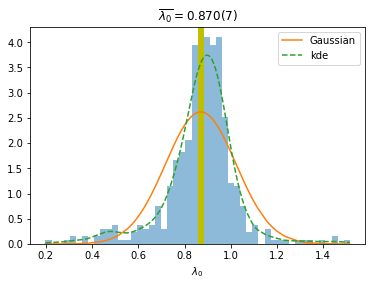
Here we plot a histogram of the data, along with a gausian distribution and a gaussian kernel-density estimate (KDE). We see that the distribution is not gaussian, but this is not a bad approximation. The yellow band shows the mean of the gaussian with a width of twice the standard error of the mean \(\delta \lambda_0 = \sigma / \sqrt{n}\) where \(\sigma\) is the standard deviation, and \(n\) is the number of samples. Note: the distribution here depends quite sensitively on dt, but the mean remains close to \(\lambda_0 = 0.87(1)\)
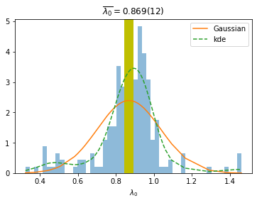
# Randomly choose some values and re-analyze:
rng = np.random.default_rng(0)
analyze(rng.choice(lams, 200))
from statsmodels.graphics.tsaplots import plot_acf
plot_acf(lams, lags=100);