Assignment 1: Monty Hall etc.¶

Assignment Preparation¶

Write a function phys_581_2021.assignment_1.play_monty_hall() which plays a single round of the standard Monty Hall problem game.

Evaluating Functions¶

Lambert W function¶

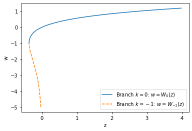
Write a function phys_581_2021.assignment_1.lambertw() that computes \(w = W_k(x)\), the Lambert W function, for the two branches \(k=0\) and \(k=-1\).

This function satisfies:

\[ z = we^w \]

and \(k\) determines which branch you should compute as shown below:

w0 = np.linspace(-1, 1.2, 100)
w1 = np.linspace(-5, -1, 100)
fig, ax = plt.subplots()
for w, k, ls in [(w0, 0, '-'), (w1, -1, '--')]:
    z = w*np.exp(w)
    ax.plot(z, w, linestyle=ls, 
            label=f"Branch $k={k}$: $w=W_{{{k}}}(z)$")
ax.legend()
ax.set(xlabel='z', ylabel='w');

Riemann zeta function¶

Write a function phys_581_2021.assignment_1.zeta() that computes the Riemann zeta function

\[ \zeta(s) = \sum_{n=1}^{\infty} \frac{1}{n^{s}}. \]

Differentiation¶

Write a function phys_581_2021.assignment_1.derivative() that numerically computes the derivatives of a function \(f(x)\) at a point \(x\):

from phys_581_2021.assignment_1 import derivative

x = 1.0
for d, exact in [
    (0, np.sin(x)),
    (1, np.cos(x)),
    (2, -np.sin(x)),
    (3, -np.cos(x)),
    (4, np.sin(x))
]:
    res = derivative(np.sin, x=x, d=d)
    rel_err = abs(res-exact)/abs(exact)
    print(f"d={d}: numeric={res:.8g}, exact={exact:.8g}, rel_err={rel_err:.4g}")

d=0: numeric=0.84147098, exact=0.84147098, rel_err=0
d=1: numeric=0.54030231, exact=0.54030231, rel_err=2.283e-11
d=2: numeric=-0.84147113, exact=-0.84147098, rel_err=1.751e-07
d=3: numeric=-0.54923415, exact=-0.54030231, rel_err=0.01653
d=4: numeric=61834.581, exact=0.84147098, rel_err=7.348e+04

The default code carefully chooses an optimal value of \(h\) as discussed below, then uses a recursive approach to compute higher derivatives. Can you improve the accuracy of this?

Bonus: Why does the following trick work to machine precision?

def derivative1(f, x):
    """Compute the first 1 derivative extremely accurately for *some* functions."""
    h = 1e-64j
    return ((f(x+h) - f(x))/h).real

print(f"f=sin(x): err = {abs(derivative1(np.sin, x) - np.cos(x))}")
print(f"f=exp(x): err = {abs(derivative1(np.exp, x) - np.exp(x))}")
f = lambda x: np.exp(-x**2)
df = lambda x: -2*x*np.exp(-x**2)
print(f"f=exp(-x**2): err = {abs(derivative1(f, x) - df(x))}")

f=sin(x): err = 0.0
f=exp(x): err = 0.0
f=exp(-x**2): err = 0.0

More Details¶

Roundoff vs Truncation Error¶

Consider computing the derivative of a function using finite-difference techniques:

\[ f'(x) = \lim_{h\rightarrow 0} \frac{f(x+h) - f(x)}{h}. \]

We can estimate the error computing this by using the Taylor series for the function:

\[\begin{split} f(x\pm h) = f(x) \pm h f'(x) + \frac{h^2}{2}f''(x) \pm \frac{h^3}{3!}f'''(x) + \sum_{n=4}^{\infty} \frac{(\pm h)^n}{n!}f^{(n)}(x),\\ D^+_h f(x) = \frac{f(x+h) - f(x)}{h} = f'(x) + \frac{h}{2}f''(x) + \order(h^2). \end{split}\]

This forward-difference approximation thus has a truncation-error that scales as \(hf''(x)/2\). We can do a bit better if we take the centered-difference approximation:

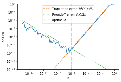
\[ D_h f(x) = \frac{f(x+h) - f(x-h)}{2h} + \frac{h^2}{6}f'''(x) + \order(h^3). \]

However, this is not the only source of error. If all goes well, the values \(f(x\pm h)\) will be computed with a relative error of machine precision \(\epsilon\), which means they will have have an absolute error of \(\approx \epsilon f(x)\). Dividing this error by \(2h\), however, means that the whole expression will have an absolute error of about \(\epsilon f(x)/2h\) because of roundoff error. Notice that this gets significantly worse as \(h\) gets small.

With this formula, the best we can do is to choose

\[ h \approx \sqrt[3]{3\epsilon \left\lvert\frac{f(x)}{f'''(x)}\right\rvert} \]

The following plot shows that these estimates are accurate.

eps = np.finfo(float).eps
h = 10 ** np.linspace(-12, 1, 100)
x = 1.0
f = np.sin
df = np.cos
d3f = lambda x: -np.sin(x)
Df_x = (f(x + h) - f(x - h)) / 2 / h  # Centered difference approx
err = abs(Df_x - df(x))
truncation_err = abs(h ** 2 * d3f(x) / 6)
roundoff_err = abs(eps * f(x) / 2 / h)
h_opt = (3*eps*abs(f(x)/d3f(x)))**(1/3)
fig, ax = plt.subplots()
ax.loglog(h, err)
ax.plot(h, truncation_err, "--", label="Truncation error: $h^2 f'''(x)/6$")
ax.plot(h, roundoff_err, ":", label="Roundoff error: $f(x)/2h$")
ax.axvline(h_opt, c='y', ls='-.', label='optimal $h$')
ax.set(xlabel="h", ylabel="abs err", ylim=(1e-16, 1))
ax.legend()

<matplotlib.legend.Legend at 0x7f8bf8fac100>

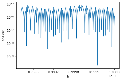
Notice that the truncation error is smooth, but the roundoff error appears random. As Alex discusses [Gezerlis, 2020] (see Fig. 2.3), roundoff errors are not random. We can see this by zooming in:

h = 10 ** np.linspace(-11, -11.0002, 1000)
Df_x = (f(x + h) - f(x - h)) / 2 / h  # Centered difference approx
err = abs(Df_x - df(x))
fig, ax = plt.subplots()
ax.semilogy(h, err)
ax.set(xlabel="h", ylabel="abs err");

Physics 581: Physics Inspired Computational Techniques

Assignment 1: Monty Hall etc.

Contents